Introduction
Rattle is a popular free and open source Graphical User Interface (GUI) for the R software, one that focuses on beginners looking to point-and-click their way through data mining tasks. Such tasks are also referred to as machine learning or predictive analytics. Rattle’s name is an acronym for “R Analytical Tool To Learn Easily.” Rattle is available on Windows, Mac, and Linux systems.
This post is one of a series of reviews which aim to help non-programmers choose the GUI that is best for them. Additionally, these reviews include a cursory description of the programming support that each GUI offers.

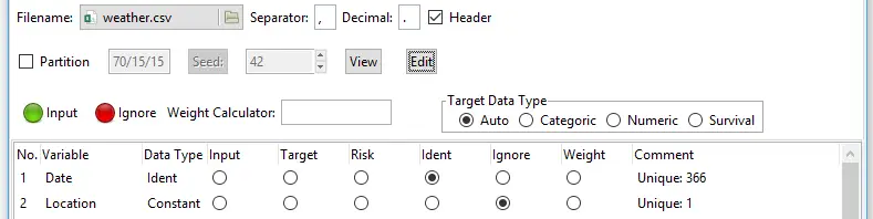
Figure 1. The Rattle interface with the “Data” tab chosen, showing which file I’m reading, and the roles of the variables will play in analyses. The role assigned to each variable is critically important. Note the all-important “Execute” button in the upper left of the screen. Nothing happens until it’s clicked.
Terminology
There are various definitions of user interface types, so here’s how I’ll be using these terms:
GUI = Graphical User Interface using menus and dialog boxes to avoid having to type programming code. I do not include any assistance for programming in this definition. So, GUI users are people who prefer using a GUI to perform their analyses. They don’t have the time or inclination to become good programmers.
IDE = Integrated Development Environment which helps programmers write code. I do not include point-and-click style menus and dialog boxes when using this term. IDE usersare people who prefer to write R code to perform their analyses.
Installation
The various user interfaces available for R differ quite a lot in how they’re installed. Some, such as jamovi or RKWard, install in a single step. Others install in multiple steps, such as R Commander (two steps) and Deducer (up to seven steps). Advanced computer users often don’t appreciate how lost beginners can become while attempting even a simple installation. The Help Desks at most universities are flooded with such calls at the beginning of each semester!
The steps to install Rattle are:
- Install R
- In R, install the toolkit that Rattle is written in by executing the command: install.packages(“RGtk2”)
- Also in R, install Rattle itself by executing the command:
install.packages(“rattle”, dependencies=TRUE)
The very latest development version is available here.
Note that while Rattle’s name is capitalized, the name of the rattle package is spelled in all lower-case letters! - If you wish to take advantage of interactive visualization (highly recommended) then install the GGobi software from: http://www.ggobi.org/downloads/.
Plug-in Modules
When choosing a GUI, one of the most fundamental questions is: what can it do for you? What the initial software installation of each GUI gets you is covered in the Graphics, Analysis, and Modeling sections of this series of articles. Regardless of what comes built-in, it’s good to know how active the development community is. They contribute “plug-ins” which add new menus and dialog boxes to the GUI. This level of activity ranges from very low (RKWard, Deducer) through moderate (jamovi) to very active (R Commander).
Rattle’s complete capability was designed and programmed by Graham Williams of Togaware. As a result, it doesn’t have plug-ins, but it does include a comprehensive set of data mining tools.
Startup
Some user interfaces for R, such as jamovi, start by double-clicking on a single icon, which is great for people who prefer to not write code. Others, such as R commander and JGR, have you start R, then load a package from your library, and call a function. That’s better for people looking to learn R, as those are among the first tasks they’ll have to learn anyway.
Rattle is run as a part of R itself, so the steps to start it begin with starting R:
- Start R.
- Load Rattle from your library by executing the command: library(“rattle”)
- Start Rattle by executing the command: rattle()
Data Editor
A data editor is a fundamental feature in data analysis software. It puts you in touch with your data and lets you get a feel for it, if only in a rough way. A data editor is such a simple concept that you might think there would be hardly any differences in how they work in different GUIs. While there are technical differences, to a beginner what matters the most are the differences in simplicity. Some GUIs, including jamovi, let you create only what R calls a data frame. They use more common terminology and call it a data set: you create one, you save one, later you open one, then you use one. Others, such as RKWard trade this simplicity for the full R language perspective: a data set is stored in a workspace. So the process goes: you create a data set, you save a workspace, you open a workspace, and choose a data set from within it.
Rattle’s data editor is unique for a GUI in that it does not offer a way to create a data set. It lets you edit any data set you open using R’s built-in edit function, but that function offers very few features. Clicking on a variable name will cause a dialog to open, offering to change the variable’s name or type as numeric or character (see Figure 2). Rattle automatically converts variables that have fewer than 10 values into “categorical” ones. R would call these factors. You can always recode variables from numeric to categorical (or vice versa) in the “Transform” tab (see Data Management section).

Figure 2. Rattle uses R’s built-in edit function as its data editor. Here I clicked on the name of the variable “Rainfall” to show how you might rename it or change its data type.
Data Import
Since R GUIs are using R to do the work behind the scenes, they often include the ability to read a wide range of files, including SAS, SPSS, and Stata. Some, like BlueSky Statistics, also include the ability to read directly from SQL databases. Of course you can always use R code to import data from any source and then continue to analyze it using any GUI, but the point of GUIs is to avoid programming.
Rattle skips many common statistical data formats, but it includes a couple exclusive ones, such as the Attribute-Relation File Format used by other data mining tools. It also includes “corpus” which reads in text documents, and it then it performs the popular tf-idfcalculation to prepare them for analysis using the other numerically-based analysis methods.
On its “Data” tab, Rattle offers several formats:
- File: CSV
- File: TXT
- File: Excel
- Attribute-Relation File Format (ARFF)
- Open Database Connectivity (ODBC)
- R Dataset
- RData File
- Library
- Corpus (for text analysis)
- Script
Data Management
It’s often said that 80% of data analysis time is spent preparing the data. Variables need to be transformed, recoded, or created; strings and dates need to be manipulated; missing values need to be handled; datasets need to be stacked or merged, aggregated, transposed, or reshaped (e.g. from wide to long and back). A critically important aspect of data management is the ability to transform many variables at once. For example, social scientists need to recode many survey items, biologists need to take the logarithms of many variables. Doing these types of tasks one variable at a time can be tedious. Some GUIs, such as jamovi and RKWard handle only a few of these functions. Others, such as BlueSky Statistics or the R Commander can handle all, or nearly all, of these tasks.
Rattle provides minimal data management tools. Its designer chose to focus on reading a single data set, and making transformations that are common in data mining projects quick and easy. More complex data management tasks are left to other tools such as SQL in a database before the data set is read in, or using R programming.
Rattle’s “Transform” tab cycles through various data management “types.” The way it works is quite unique. As you can see in Figure X, I have selected the Transform tab by clicking on it. I then held the CTRL key down to select several variables that are highlighted in blue. If the variables had been next to one another, I could have clicked on the first one, then shift-clicked on the last to select them all. Next I chose my transformation, by choosing “Recode” and then “Recenter.” Finally, I clicked the “Execute” button (or F2) to complete the process by adding three new recoded variables to the data set. Original variables are never changed, and you never have the ability to choose the name of the new variable(s). A prefix is appended to the variable name(s) automatically to speed the process. In this case, my Rainfall variable was transformed into “RRC_Rainfall”. The RRC prefix stands for “Recoded, Re-Centered.”
Whenever a variable is transformed, its status in the “Data” tab switches from “Input” to “Ignore”, while the transformed version of variable enters the data with an “Input” role.
![]()
Figure 3. Rattle’s “Transform” tab with three variables selected. The “Recode” sub-tab is also selected and the “Recenter” transformation is chosen. When the “Explore” button is clicked, the newly tranformed variables will be appended to the data set with a prefix indicating the type of transformation performed.
As easy as some transformations are, other transformations are impossible. For example, if you had a formula to calculate recommended daily allowances of vitamins, there’s no way to do it. Conditional transformations, those which have different formulas for different subsets of the observations (e.g. daily allowances of vitamins calculated differently for men and women) are also not possible. Here are the available transformations:
Transform> Rescale> Normalize
- Recenter (Z-score)
- Scale 0 to 1
- (Var – Median)/Mean Absolute Deviation (MAD)
- Natural Log
- Log 10
- Matrix (divide all by a constant)
Transform> Impute
- Replace missing with zeros (e.g. requesting nothing gets you nothing)
- Mean
- Median
- Mode
- Constant
Transform> Recode
- Binning> Quantiles
- Binning> KMeans clusters
- Binning> Equal width intervals
- Binning> N Equally spaced intervals
- Indicator variables
- Join Categorics
- As Categoric
- As Numeric
Continued here…