by Robert A. Muenchen, updated 2/8/2023
Introduction
JASP is a free and open-source statistics package that targets beginners looking to point-and-click their way through analyses. This article is one of a series of reviews that aim to help non-programmers choose the Graphical User Interface (GUI) for R which best meets their needs. Most of these reviews also include cursory descriptions of the programming support that each GUI offers.
I have joined the BlueSky Statistics development team and have written the BlueSky User Guide (online here), but you can trust this series of reviews, as I describe here. All my comments below are easily verifiable. There is no perfect user interface for everyone; each GUI for R has features that appeal to different people.
JASP stands for Jeffreys’ Amazing Statistics Program, a nod to the Bayesian statistician Sir Harold Jeffreys. It is available for Windows, Mac, and Linux, and there is even a cloud version. One of JASP’s key features is its emphasis on Bayesian analysis. Most statistics software emphasizes a more traditional frequentist approach; JASP offers both. However, while JASP uses R to do some of its calculations, it does not currently show you the R code it uses, nor does it allow you to execute your own. The developers hope to add that to a future version. Some of JASP’s calculations are done in C++, so getting that converted to R will be a necessary first step on that path.
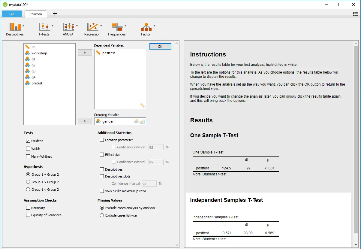
Figure 1. JASP’s main screen.
Terminology
There are various definitions of user interface types, so here’s how I’ll be using the following terms. Reviewing R GUIs keeps me quite busy, so I don’t have time also to review all the IDEs, though my favorite is RStudio.
GUI = Graphical User Interface using menus and dialog boxes to avoid having to type programming code. I do not include any assistance for programming in this definition. So, GUI users are people who prefer using a GUI to perform their analyses. They don’t have the time or inclination to become good programmers.
IDE = Integrated Development Environment, which helps programmers write code. I do not include point-and-click style menus and dialog boxes when using this term. IDE users are people who prefer to write R code to perform their analyses.
Reproducibility = The ability to record and re-run every detail of an analysis, preferably integrated with the text that describes those results. Most of the R GUIs offer code reproducibility, the ability to record the R code that you can use to reproduce the workflow. However, GUI users often don’t understand the code and have trouble re-purposing it for similar analyses. GUI reproducibility is the ability to save the workflow in GUI form. That is usually the dialog boxes and their settings that created the original complete analysis.
Installation
The various user interfaces available for R differ quite a lot in how they’re installed. Some, such as BlueSky Statistics, jamovi, and RKWard, install in a single step. Others install in multiple steps, such as R Commander (two steps) and Deducer (up to seven steps). Advanced computer users often don’t appreciate how lost beginners can become while attempting even a simple installation. The HelpDesks at most universities are flooded with such calls at the beginning of each semester!
JASP’s single-step installation is extremely easy and includes its own copy of R. So, if you already have a copy of R installed, you’ll have two after installing JASP. That’s a good idea, though, as it guarantees compatibility with the version of R that it uses, plus a standard R installation by itself is harder than JASP’s.
Plug-in Modules
When choosing a GUI, one of the most fundamental questions is: what can it do for you? What the initial software installation of each GUI gets you is covered in the Graphics, Analysis, and Modeling sections of this series of articles. Regardless of what comes built-in, it’s good to know how active the development community is. They contribute “plug-ins” that add new menus and dialog boxes to the GUI. This level of activity ranges from very low (Deducer, RKWard) to very high (BlueSky, R Commander).
For JASP, plug-ins are called “modules,” and they are found by clicking the “+” sign at the top of its main screen. That causes a new menu item to appear. However, unlike most other software, the menu additions are not saved when you exit JASP; you must add them every time you wish to use them.
JASP’s modules are currently included with the software’s main download. However, future versions will store them in their own repository rather than on the Comprehensive R Archive Network (CRAN) where R and most of its packages are found. This makes locating and installing JASP modules especially easy.
Currently, there are fourteen add-on modules for JASP:
- AUDIT
- BAIN
- Circular Statistics
- Distributions
- Equivalence T-Tests
- JAGS
- Learn Bayes
- Machine Learning
- Meta-Analysis
- Network Analysis
- Prophet
- Reliability
- Summary Stats – provides variations on the methods included in the Common menu
- SEM – Structural Equation Modeling using lavaan (this is more of a window in which you type R code than a GUI dialog)
- Visual Modeling
Startup
Some user interfaces for R, such as BlueSky, jamovi, and Rkward, start by double-clicking on a single icon, which is great for people who prefer to not write code. Others, such as R commander and Deducer, have you start R, then load a package from your library, and then call a function to finally activate the GUI. That’s more appropriate for people looking to learn R, as those are among the first tasks they’ll have to learn anyway.
You start JASP directly by double-clicking its icon from your desktop or choosing it from your Start Menu (i.e. not from within R itself). It interacts with R in the background; you never need to be aware that R is running.
Data Editor
A data editor is a fundamental feature in data analysis software. It puts you in touch with your data and lets you get a feel for it, if only in a rough way. A data editor is such a simple concept that you might think there would be hardly any differences in how they work in different GUIs. While there are technical differences, to a beginner what matters the most are the differences in simplicity. Some GUIs, including BlueSky and jamovi, let you create only what R calls a data frame. They use more common terminology and call it a data set: you create one, you save one, later you open one, then you use one. Others, such as RKWard trade this simplicity for the full R language perspective: a data set is stored in a workspace. So the process goes: you create a data set, you save a workspace, you open a workspace, and choose a dataset from within it.
JASP is the only program in this set of reviews that lacks a data editor. It has only a data viewer (Figure 2, left). If you point to a cell, a message pops up to say, “double-click to edit data” and doing so will transfer the data to another program where you can edit it. You can choose which program will be used to edit your data in the “Preferences>Data Editing” tab, located under the “hamburger” menu in the upper-right corner. The default is Excel.
When JASP opens a data file, it automatically assigns metadata to the variables. As you can see in Figure 2, it has decided my variable “pretest” was a factor and provided a bar chart showing the counts of every value. For the extremely similar “posttest” variable it decided it was numeric, so it binned the values and provided a more appropriate histogram.
While JASP lacks the ability to edit data directly, it does allow you to edit some of the metadata, such as variable scale and variable (factor levels). I fixed the problem described above by clicking on the icon to the left of each variable name, and changing it from a Venn diagram representing “nominal”, to a ruler for “scale”. Note the use of terminology here, which is statistical rather than based on R’s use of “factor” and “numeric” abxyxas respectively. Teaching R is not part of JASP’s mission.
JASP cannot handle date/time variables other than to read them as characters and convert them to factors. Once JASP decides a character or date/time variable is a factor, it cannot be changed.
Clicking on the name of a factor will open a small window on the top of the data viewer where you can overwrite the existing labels. Variable names however, cannot be changed without going back to Excel, or whatever editor you used to enter the data.
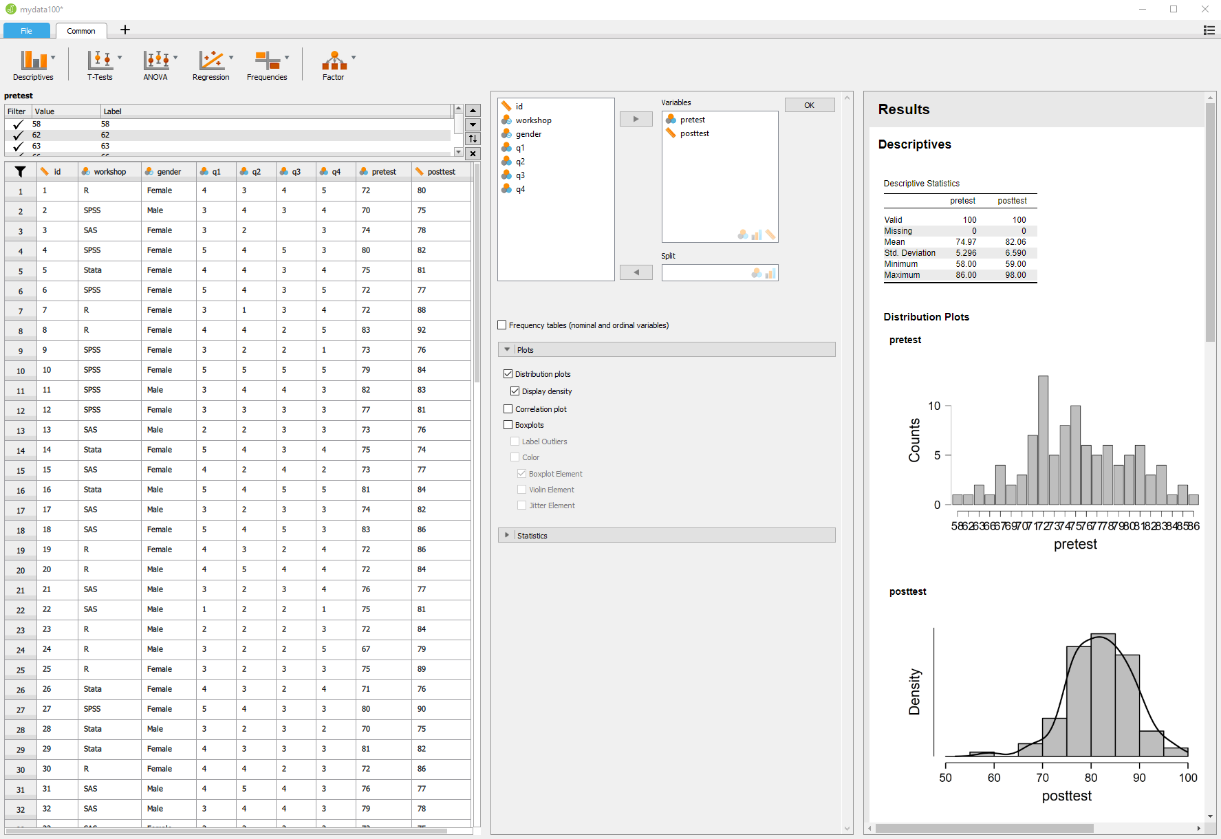
Figure 2. The JASP data viewer is shown on the left-hand side.
Data Import
The ability to import data from a wide variety of formats is extremely important; you can’t analyze what you can’t access. Most of the GUIs evaluated in this series can open a wide range of file types and even pull data from relational databases. JASP can’t read data from databases, but it can import the following file formats. Though based on R, JASP cannot read R data files!
- Comma Separated Values (.csv)
- Plain text files (.txt)
- SAS
- SPSS (.sav, but not .zsav, .por)
- Stata
- Open Document Spreadsheet (.ods)
Data Export
The ability to export data to a wide range of file types helps when you need multiple tools to complete a task. Research is commonly a team effort, and in my experience, it’s rare to have all team members prefer to use the same tools. For these reasons, GUIs such as BlueSky, Deducer, and jamovi offer many export formats. Others, such as R Commander and RKward can create only delimited text files.
A fairly unique feature of JASP is that it doesn’t save just a dataset, but instead it saves the combination of a dataset plus its associated analyses. To save just the dataset, you go to the “File” tab and choose “Export Data.” The only export format is a comma-separated value file (.csv).
Data Management
It’s often said that 80% of data analysis time is spent preparing the data. Variables need to be computed, transformed, scaled, recoded, or binned; strings and dates need to be manipulated; missing values need to be handled; datasets need to be sorted, stacked, merged, aggregated, transposed, or reshaped (e.g. from “wide” format to “long” and back).
A critically important aspect of data management is the ability to transform many variables at once. For example, social scientists need to recode many survey items, biologists need to take the logarithms of many variables. Doing these types of tasks one variable at a time is tedious.
Some GUIs, such as BlueSky and R Commander, can handle nearly all of these tasks. Others, such as jamovi and RKWard handle only a few of these functions.
JASP’s data management capabilities are minimal. It has a simple calculator that works by dragging and dropping variable names and math or statistical operators. Alternatively, you can type formulas using R code. Using this approach, you can only modify one variable at time, making day-to-day analysis quite tedious. It’s also unable to apply functions across rows (jamovi handles this via a set of row-specific functions). Using the calculator, I could never figure out how to later edit the formula or even delete a variable if I made an error. I tried to recreate one, but it told me the name was already in use.
You can filter cases to work on a subset of your data. However, JASP can’t sort, stack, merge, aggregate, transpose, or reshape datasets. The lack of combining datasets may be a result of the fact that JASP can only have one dataset open in a given session.
Menus & Dialog Boxes
The goal of pointing and clicking your way through an analysis is to save time by recognizing menu settings rather than performing the more difficult task of recalling programming commands. Some GUIs, such as BlueSky and jamovi, make this easy by sticking to menu standards and using simpler dialog boxes; others, such as RKWard, use non-standard menus that are unique to it and hence require more learning.
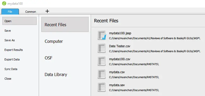
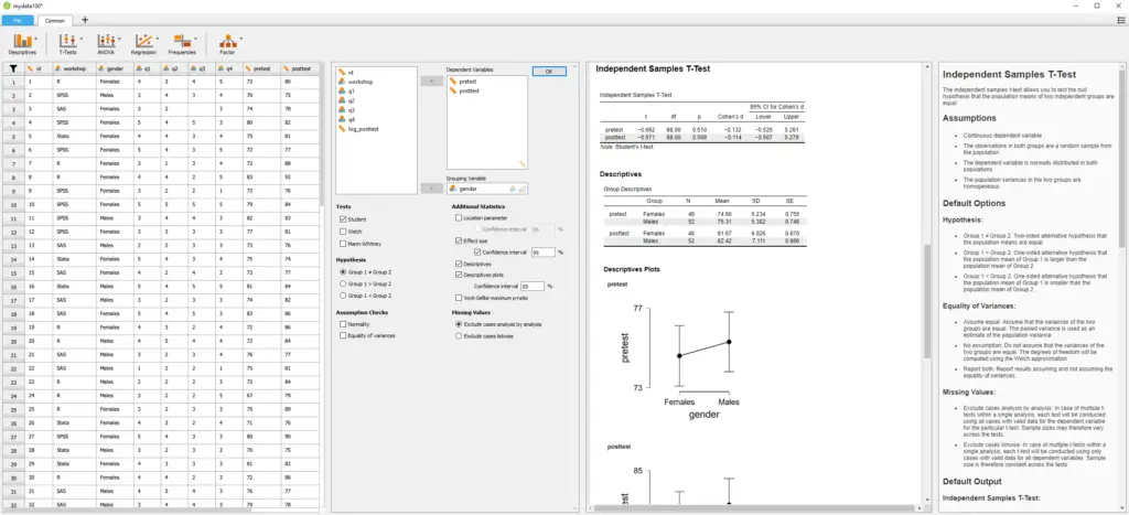
JASP’s interface uses tabbed windows and toolbars in a way that’s similar to Microsoft Office. As you can see in Figure 3, the “File” tab contains what is essentially a menu, but it’s already in the dropped-down position so there’s no need to click on it. Depending on your selections there, a side menu may pop out, and it stays out without holding the mouse button down.
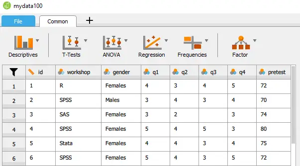
The built-in set of analytic methods are contained under the “Common” tab. Choosing that yields a shift from menus to toolbar icons shown in Figure 4.
Clicking on any icon on the toolbar causes a standard dialog box to pop out the right side of the data viewer (Figure 2, center). You select variables to place into their various roles. This is accomplished by either dragging the variable names or by selecting them and clicking an arrow located next to the particular role box. As soon as you fill in enough options to perform an analysis, its output appears instantly in the output window to the right. Thereafter, every option chosen adds to the output immediately; every option turned off removes output. The dialog box does have an “OK” button, but rather than cause the analysis to run, it merely hides the dialog box, making room for more space for the data viewer and output. Clicking on the output itself causes the associated dialog to reappear, allowing you to make changes.
While nearly all GUIs keep your dialog box settings during your session, JASP keeps those settings in its main file. This allows you to return to a given analysis at a future date and try some model variations. You only need to click on the output of any analysis to have the dialog box appear to the right of it, complete with all settings intact.
Output is saved by using the standard “File> Save” selection.
Documentation & Training
The JASP Materials web page provides links to a helpful array of information to get you started. The How to Use JASP web page offers a cornucopia of training materials, including blogs, GIFs, and videos. The free book, Statistical Analysis in JASP: A Guide for Students, covers the basics of using the software and includes a basic introduction to statistical analysis.
Help
R GUIs provide simple task-by-task dialog boxes which generate much more complex code. So for a particular task, you might want to get help on 1) the dialog box’s settings, 2) the custom functions it uses (if any), and 3) the R functions that the custom functions use. Nearly all R GUIs provide all three levels of help when needed. The notable exception is the R Commander, which lacks help on the dialog boxes themselves.
JASP’s help files are activated by choosing “Help” from the hamburger menu in the upper right corner of the screen (Figure 5). When checked, a window opens on the right of the output window, and its contents change as you scroll through the output. Given that everything appears in a single window, having a large screen is best.
The help files are very well done, explaining what each choice means, its assumptions, and even journal citations. While there is no reference to the R functions used, nor any link to their help files, the overall set of R packages JASP uses is listed here.
Graphics
The various GUIs available for R handle graphics in several ways. Some, such as RKWard, focus on R’s built-in graphics. Others, such as BlueSky, focus on R’s popular ggplot graphics. GUIs also differ quite a lot in how they control the style of the graphs they generate. Ideally, you could set the style once, and then all graphs would follow it.
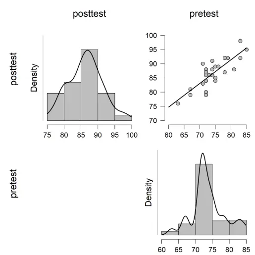
There is no “Graphics” menu in JASP; all the plots are created from within the data analysis dialogs. For example, boxplots are found in “Common> Descriptives> Plots.” To get a scatterplot I tried “Common> Regression> Plots” but only residual plots are found there. Next, I tried “Common> Descriptives> Plots> Correlation plots” and was able to create the image shown in Figure 6. Apparently, there is no way to get just a single scatterplot.
The plots JASP creates are well done, with a white background and axes that don’t touch at the corners. It’s unclear which R functions are used to create them as their style is not the default from the R’s default graphics package, ggplot2, or lattice.
The most important graphical ability that JASP lacks is the ability to do “small multiples” or “facets”. Faceted plots allow you to compare groups by showing a set of the same type of plot repeated by levels of a categorical variable.
Setting the dots-per-inch is the only graphics adjustment JASP offers. It doesn’t support styles or templates. However, plot editing is planned for a future release.
Here is the selection of plots JASP can create.
- Histogram
- Density
- Box Plots
- Bar Plots
- Confidence intervals
- Machine Learning: Data Split
- Machine Learning: Out-of-bag Improvement
- Machine Learning: ROC Curves
- Machine Learning: Andrews Curves
- Machine Learning: Deviance
- Machine Learning: Relative Influence
- Machine Learning: Decision Boundary Matrix Plot
- Network: Network Plot
- Network: Centrality Plot
- Network: Clustering Plot
- Scatterplot matrix
- Scatter – of residuals
- SEM Path Diagrams
- Strip Plots
- Violin Plots
Modeling
The way statistical models (which R stores in “model objects”) are created and used is an area in which R GUIs differ the most. Some, like RKWard, use a one-step approach to modeling. That approach tries to do everything you might need in a single dialog box. This is perfect for beginners who appreciate being reminded of the various assumption tests and evaluation steps to take. But to an R programmer, that approach seems confining since R can do a lot of different tasks with model objects. However, neither SAS nor SPSS were able to save models for their first 35 years of existence, so each approach has its merits. For simple models like linear regression, standard compute statements can enter models to make predictions. Entering them manually is not much effort, and it saves you from having to learn what a model object is. However, some of the most powerful model types are essentially impossible to enter by hand, such as neural networks, random forests, and gradient-boosting machines.
Other GUIs, such as BlueSky and R Commander, do modeling using a two-step process. First, you generate and save a model, then use it for scoring new datasets, calculating model-level measures of fit or observation-level scores of influence, diagnostic plotting, testing differences between models, and so on.
JASP follows the one-step approach. It does not save models in its base package, so you need to use compute statements to enter a model and apply it to a new data set (or a hold-out sample) to see how effectively the model generalizes. Instead, it tries to anticipate your needs, providing things like normal probability plots for residuals. This is great for intro statistics courses, but it lacks the flexibility that more advanced researchers might prefer. JASP has an add-on module for machine learning that does offer a way to save models. Perhaps JASP’s internal modeling functions will eventually work in a similar fashion.
Another way in which R GUIs differ is the model formula builder. Some, like jamovi and RKWard, offer only the most popular model types, providing interactions and allowing you to force the y-intercept through zero. Others, such as R Commander and BlueSky, offer maximum power by including buttons to control nested factors, polynomials, splines, and so on.
JASP’s base modeling keeps model formulas simple. It adds the variables you select, and all their possible interactions. That can generate a warning that you don’t have enough degrees of freedom, allowing you to remove terms then. Since JASP’s model builder does not offer advanced features like nested effects and splines, those types of models cannot be done. The model it builds is not displayed as a standard R formula which you could modify manually.
JASP 0.17 has problems modeling with large datasets. While I have not determined at what level the problem starts, a linear regression on a million variables locks the software up. All of the other R GUIs are capable of analyzing far more data. I have reported the problem, and the JASP development team is working on it.
Analysis Methods
All of the R GUIs offer a decent set of statistical analysis methods. Some also offer machine learning methods. As you can see from the table below, JASP offers both. Included in many of these are Bayesian measures, such as credible intervals. See the Plug-in Modules section above for more analysis types.
Generated R Code
One of the aspects that most differentiates the various GUIs for R is the code they generate. If you decide you want to save code, what type of code is best for you? The base R code as provided by the R Commander which can teach you “classic” R? The tidyverse code generated by BlueSky Statistics? The completely transparent (and complex) traditional code provided by RKWard, which might be the best for budding R power users?
JASP uses R code behind the scenes, but it does not show it to you. There is no way to extract that code to run in R by itself. The JASP developers have that on their to-do list.
Support for Programmers
Some of the GUIs reviewed in this series of articles include extensive support for programmers. For example, RKWard offers much of the power of Integrated Development Environments (IDEs) such as RStudio or Eclipse StatET. Others, such as jamovi or the R Commander, offer just a text editor with some syntax checking and code completion suggestions.
JASP’s code editor is tiny at only four lines long. It offers no syntax checking or code completion, and you can only submit one function call at a time.
Reproducibility & Sharing
One of the biggest challenges that GUI users face is being able to reproduce their work. Reproducibility is useful for re-running everything on the same dataset if you find a data entry error. It’s also useful for applying your work to new datasets so long as they use the same variable names (or the software can handle name changes). Some scientific journals ask researchers to submit their files (usually code and data) along with their written reports so that others can check their work.
As important a topic as it is, reproducibility is a problem for GUI users, a problem that has only recently been solved by some software developers. Most GUIs (e.g. the R Commander, Rattle) save only code, but since GUI users don’t write the code, they also can’t read it or change it! Others, such as BlueSky, jamovi, and RKWard, save the dialog box entries and allow GUI users to have reproducibility in the form they prefer.
JASP records the steps of all analyses, providing exact reproducibility. In addition, if you update a data value, all the analyses that used that variable are recalculated instantly. That’s a very useful feature since people coming from Excel expect this to happen. You can also use “File> Sync Data” to open a new data file and rerun all analyses on that new dataset. However, the dataset must have exactly the same variable names in the same order for this to work. Still, it’s a very feature that GUI users will find very useful.
If you wish to share your work with a colleague so they too can execute it, they must be JASP users. There is no way to export an R program file for them to use. You need to send them only your JASP file; It contains both the data and the steps you used to analyze it.
Package Management
A topic related to reproducibility is package management. One of the major advantages of the R language is that it’s very easy to extend its capabilities through add-on packages. However, updates in these packages may break a previously functioning analysis. Years from now, you may need to run a variation of an analysis, which would require you to find the version of R you used, plus the packages you used at the time. As a GUI user, you’d also need to find the version of the GUI that was compatible with that version of R.
Some GUIs, such as the R Commander and Deducer, depend on you to find and install R. For them, the problem is left for you to solve. Others, such as BlueSky, distribute their own version of R, all R packages, and all of its add-on modules. This requires a bigger installation file, but it makes dealing with long-term stability as simple as finding the version you used when you last performed a particular analysis. Of course, this depends on all major versions being around for the long term, but for open-source software, there are usually multiple archives available to store software even if the original project is defunct.
JASP if firmly in the latter camp. It provides nearly everything you need in a single download. This includes the JASP interface, R itself, and all R packages that it uses. So for the base package, you’re all set.
Output & Report Writing
Ideally, output should be clearly labeled, well organized, and of publication quality. It might also delve into the realm of word processing through R Markdown, knitr or Sweave documents. At the moment, none of the GUIs covered in this series of reviews meets all of these requirements. See the separate reviews to see how each other package is doing on this topic.
The labels for each of JASP’s analyses are provided by a single main title which is editable, and subtitles, which are not. Pointing at a title will cause a black triangle to appear, and clicking that will drop a menu down to edit the title (the single main one only) or to add a comment below (possible with all titles).
You can adjust the output by deleting sections or by moving them around.
JASP has a table of contents (TOC) feature that is extremely well done. Each step in your analysis appears in the TOC automatically. Clicking on its entry drops the dialog down into view where you can change and rerun it. You can also change the order of the steps by simply dragging their titles around. This is the most well-done TOC of any of the R GUIs I have reviewed. I hope the others follow JASP’s lead on this.
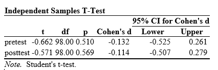
JASP’s output quality is very high, with nice fonts and true rich text tables (Table 2). Tabular output is displayed in the popular style of the American Psychological Association. That means you can right-click on any table and choose “Copy,” and the formatting is retained. That really helps speed your work as R output defaults to mono-spaced fonts that require additional steps to get into publication form (e.g. using functions from packages such as xtable or texreg). You can also export an entire set of analyses to HTML, then open the nicely-formatted tables in Word.
LaTeX users can right-click on any output table and choose “Copy special> LaTeX code” to recreate the table in that text formatting language.
Group-By Analyses
Repeating an analysis on different groups of observations is a core task in data science. Software needs to provide an ability to select a subset one group to analyze, then another subset to compare it to. All the R GUIs reviewed in this series can do this task. JASP offers a funnel icon located in the upper left corner of the data viewer. Clicking it opens a window that allows you to use icons of logical symbols to build your selection logic, such as “gender = Female.” That saves beginners from knowing that R uses “==” for logical equivalence. Nor do beginners need to know to enclose strings in quotes. Alternately, you can type a filter using R code. Either way, it generates a subset that you can analyze in the same way as the entire dataset. Second, you can click on the name of a factor, then check or un-check the values you wish to keep. Either way, the data viewer grays out the excluded data lines to give you a visual cue.
Software also needs the ability to automate such selections so that you might generate dozens of analyses, one group at a time. While this has been available in commercial GUIs for decades (e.g. SPSS “split-file,” SAS “by” statement), BlueSky is the only R GUI reviewed here that includes this feature. The closest JASP gets on this topic is to offer a “split” variable selection box in its Descriptives procedure.
Output Management
Early in the development of statistical software, developers tried to guess what output would be important to save to a new dataset (e.g. predicted values, factor scores), and the ability to save such output was built into the analysis procedures themselves. However, researchers were far more creative than the developers anticipated. To better meet their needs, output management systems were created and tacked on to existing tools (e.g. SAS’ Output Delivery System, SPSS’ Output Management System). One of R’s greatest strengths is that every bit of output can be readily used as input. However, with the simplification that GUIs provide that’s a challenge.
Output data can be observation-level, such as predicted values for each observation or case. When group-by analyses are run, the output data can also be observation-level, but now the (e.g.) predicted values would be created by individual models for each group, rather than one model based on the entire original data set (perhaps with group included as a set of indicator variables).
You can also use group-by analyses to create model-level data sets, such as one R-squared value for each group’s model. You can also create parameter-level data sets, such as the p-value for each regression parameter for each group’s model. (Saving and using single models is covered under “Modeling” above.)
For example, in our organization, we have 250 departments and want to see if any have a gender bias on salary. We write all 250 regression models to a dataset and then search to find those whose gender parameter is significant (hoping to find none, of course!)
BlueSky is the only R GUI reviewed here that does all three levels of output management. JASP not only lacks these three levels of output management, it even lacks the fundamental observation-level saving that SAS and SPSS offered in their first versions back in the early 1970s. This entails saving predicted values or residuals from regression, scores from principal components analysis, or factor analysis.
Developer Issues
While most of the R GUI projects encourage module development by volunteers, the JASP project hasn’t done so. However, this is planned for a future release.
Conclusion
JASP is easy to learn and use. The tables and graphs it produces follow the guidelines of the Americal Psychological Association, making them acceptable by many scientific journals without any additional formatting. Its table of contents makes quick work of restructuring a report. Its developers have chosen their options carefully so that each analysis includes what a researcher would want to see. Its coverage of Bayesian methods is the most extensive I’ve seen in this series of software reviews. Only jamovi offers a similar set, since its developers copied the same code from JASP to jamovi.
As nice as JASP is, it lacks important features, including: a data editor, a full R code editor, the ability to see the R code it writes, the ability to handle date/time variables, the ability to perform many more fundamental data management tasks, the ability to save new variables such as predicted values or factor scores, the ability to create nested or spline models, and the ability to save models so they can be tested on hold-out samples or new data sets.
Acknowledgments
Thanks to Eric-Jan Wagenmakers and Bruno Boutin for their help in understanding JASP’s finer points. Thanks also to Rachel Ladd, Ruben Ortiz, Christina Peterson, and Josh Price for their editorial suggestions. Edit