Sooner or later, most R programmers end up with code that no longer runs because of package updates. One way to address the problem was the MRAN Time Machine which Microsoft retired on July 1, 2023. You can get similar functionality for source packages using “dateback,” thanks to Ryota Suzuki. As with MRAN, examples of when you could benefit from using dateback include:
Checking the reproducibility of old code without pre-archived R packages.
Returning your code to an older state when everything was fine.
Needing to work on an older version of R, on which recent versions of some packages do not work properly (or cannot be installed) due to compatibility issues.
Needing source package files to make a Docker image stable and reproducible, especially when using an older version of R.
Let’s consider an example. There are three options to install a source package, “ranger.”
They ALL get “ranger” and its dependencies (Rcpp and RcppEigen). The differences are:
CRAN provides the latest versions, some of which were released AFTER 2023-03-01 (ranger 0.15.1 released on 2023-04-03, and Rcpp 1.0.11 released on 2023-07-06).
With MRAN Time Machine, we could get the desired versions (ranger 0.14.1 released on 2022-06-18, and Rcpp 1.0.10 released on 2023-01-22). We could also get the binary versions, but the site is now shut down.
dateback gets basically the same versions as MRAN Time Machine, including dependencies (some may slightly differ since we don’t have the exact snapshot of CRAN, but they should be almost identical).
Of course, we can manually search on CRAN and find desired versions. But it makes a huge difference when we install a package with many complicated dependencies (like a package X depends on Y and Z, Y depends on P and Q, and so on). The number of packages needed can run into the dozens. With dateback, you don’t need to worry about what they are or how many.
Ryota is also the lead developer for R AnalyticFlow, the only workflow-style graphical user interface for R. You can download that for free here and read my review of it here. How it compares to other R GUIs is summarized here. Thanks to Ryota for most of the information in this post!
Are attending this year’s Joint Statistical Meetings in Toronto? If so, stop by booth 404 to see the latest features of BlueSky Statistics. A menu-based graphical user interface for the R language, BlueSky lets people access the power of R without having to learn to program. Programmers can easily add code to BlueSky’s menus, sharing their expertise with non-programmers. My detailed review of BlueSky is here, a brief comparison to other R GUIs is here, and the BlueSky User Guide is here. I hope to see you in Toronto!
I’ve updated The Popularity of Data Science Software‘s market share estimates based on scholarly articles. I posted it below, so you don’t have to sift through the main article to read the new section.
Scholarly Articles
Scholarly articles provide a rich source of information about data science tools. Because publishing requires significant effort, analyzing the type of data science tools used in scholarly articles provides a better picture of their popularity than a simple survey of tool usage. The more popular a software package is, the more likely it will appear in scholarly publications as an analysis tool or even as an object of study.
Since scholarly articles tend to use cutting-edge methods, the software used in them can be a leading indicator of where the overall market of data science software is headed. Google Scholar offers a way to measure such activity. However, no search of this magnitude is perfect; each will include some irrelevant articles and reject some relevant ones. The details of the search terms I used are complex enough to move to a companion article, How to Search For Data Science Articles.
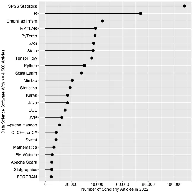
Figure 2a shows the number of articles found for the more popular software packages and languages (those with at least 4,500 articles) in the most recent complete year, 2022.
Figure 2a. The number of scholarly articles found on Google Scholar for data science software. Only those with more than 4,500 citations are shown.
SPSS is the most popular package, as it has been for over 20 years. This may be due to its balance between power and its graphical user interface’s (GUI) ease of use. R is in second place with around two-thirds as many articles. It offers extreme power, but as with all languages, it requires memorizing and typing code. GraphPad Prism, another GUI-driven package, is in third place. The packages from MATLAB through TensorFlow are roughly at the same level. Next comes Python and Scikit Learn. The latter is a library for Python, so there is likely much overlap between those two. Note that the general-purpose languages: C, C++, C#, FORTRAN, Java, MATLAB, and Python are included only when found in combination with data science terms, so view those counts as more of an approximation than the rest. Old stalwart FORTRAN appears last in this plot. While its count seems close to zero, that’s due to the wide range of this scale, and its count is just over the 4,500-article cutoff for this plot.
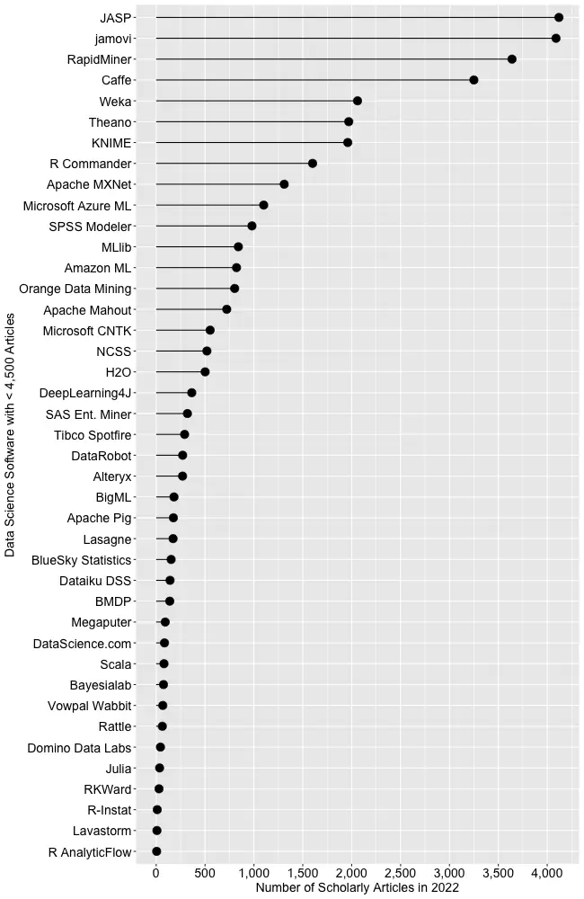
Continuing on this scale would make the remaining packages appear too close to the y-axis to read, so Figure 2b shows the remaining software on a much smaller scale, with the y-axis going to only 4,500 rather than the 110,000 used in Figure 2a. I chose that cutoff value because it allows us to see two related sets of tools on the same plot: workflow tools and GUIs for the R language that make it work much like SPSS.
Figure 2b. Number of scholarly articles using each data science software found using Google Scholar. Only those with fewer than 4,500 citations are shown.
JASP and jamovi are both front-ends to the R language and are way out front in this category. The next R GUI is R Commander, with half as many citations. Still, that’s far more than the rest of the R GUIs: BlueSky Statistics, Rattle, RKWard, R-Instat, and R AnalyticFlow. While many of these have low counts, we’ll soon see that the use of nearly all is rapidly growing.
Workflow tools are controlled by drawing 2-dimensional flowcharts that direct the flow of data and models through the analysis process. That approach is slightly more complex to learn than SPSS’ simple menus and dialog boxes, but it gets closer to the complete flexibility of code. In order of citation count, these include RapidMiner, KNIME, Orange Data Mining, IBM SPSS Modeler, SAS Enterprise Miner, Alteryx, and R AnalyticFlow. From RapidMiner to KNIME, to SPSS Modeler, the citation rate approximately cuts in half each time. Orange Data Mining comes next, at around 30% less. KNIME, Orange, and R Analytic Flow are all free and open-source.
While Figures 2a and 2b help study market share now, they don’t show how things are changing. It would be ideal to have long-term growth trend graphs for each software, but collecting that much data is too time-consuming. Instead, I’ve collected data only for the years 2019 and 2022. This provides the data needed to study growth over that period.
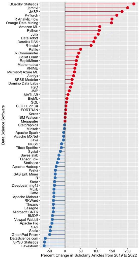
Figure 2c shows the percent change across those years, with the growing “hot” packages shown in red (right side) and the declining or “cooling” ones shown in blue (left side).
Figure 2c. Change in Google Scholar citation rate from 2019 to the most recent complete year, 2022. BlueSky (2,960%) and jamovi (452%) growth figures were shrunk to make the plot more legible.
Seven of the 14 fastest-growing packages are GUI front-ends that make R easy to use. BlueSky’s actual percent growth was 2,960%, which I recoded as 220% as the original value made the rest of the plot unreadable. In 2022 the company released a Mac version, and the Mayo Clinic announced its migration from JMP to BlueSky; both likely had an impact. Similarly, jamovi’s actual growth was 452%, which I recoded to 200. One of the reasons the R GUIs were able to obtain such high percentages of change is that they were all starting from low numbers compared to most of the other software. So be sure to look at the raw counts in Figure 2b to see the raw counts for all the R GUIs.
The most impressive point on this plot is the one for PyTorch. Back on 2a we see that PyTorch was the fifth most popular tool for data science. Here we see it’s also the third fastest growing. Being big and growing fast is quite an achievement!
Of the workflow-based tools, Orange Data Mining is growing the fastest. There is a good chance that the next time I collect this data Orange will surpass SPSS Modeler.
The big losers in Figure 2c are the expensive proprietary tools: SPSS, GraphPad Prism, SAS, BMDP, Stata, Statistica, and Systat. However, open-source R is also declining, perhaps a victim of Python’s rising popularity.
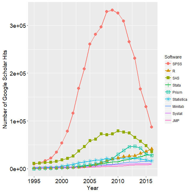
I’m particularly interested in the long-term trends of the classic statistics packages. So in Figure 2d, I have plotted the same scholarly-use data for 1995 through 2016.
Figure 2d. The number of Google Scholar citations for each classic statistics package per year from 1995 through 2016.
SPSS has a clear lead overall, but now you can see that its dominance peaked in 2009, and its use is in sharp decline. SAS never came close to SPSS’s level of dominance, and its usage peaked around 2010. GraphPad Prism followed a similar pattern, though it peaked a bit later, around 2013.
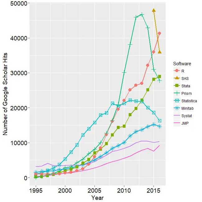
In Figure 2d, the extreme dominance of SPSS makes it hard to see long-term trends in the other software. To address this problem, I have removed SPSS and all the data from SAS except for 2014 and 2015. The result is shown in Figure 2e.
Figure 2e. The number of Google Scholar citations for each classic statistics package from 1995 through 2016, with SPSS removed and SAS included only in 2014 and 2015. The removal of SPSS and SAS expanded scale makes it easier to see the rapid growth of the less popular packages.
Figure 2e shows that most of the remaining packages grew steadily across the time period shown. R and Stata grew especially fast, as did Prism until 2012. The decline in the number of articles that used SPSS, SAS, or Prism is not balanced by the increase in the other software shown in this graph.
These results apply to scholarly articles in general. The results in specific fields or journals are likely to differ.
You can read the entire Popularity of Data Science Software here; the above discussion is just one section.
I have recently updated my extensive analysis of the popularity of data science software. This update covers perhaps the most important section, the one that measures popularity based on the number of job advertisements. I repeat it here as a blog post, so you don’t have to read the entire article.
Job Advertisements
One of the best ways to measure the popularity or market share of software for data science is to count the number of job advertisements that highlight knowledge of each as a requirement. Job ads are rich in information and are backed by money, so they are perhaps the best measure of how popular each software is now. Plots of change in job demand give us a good idea of what will become more popular in the future.
Indeed.com is the biggest job site in the U.S., making its collection of job ads the best around. As their co-founder and former CEO Paul Forster stated, Indeed.com includes “all the jobs from over 1,000 unique sources, comprising the major job boards – Monster, CareerBuilder, HotJobs, Craigslist – as well as hundreds of newspapers, associations, and company websites.” Indeed.com also has superb search capabilities.
Searching for jobs using Indeed.com is easy, but searching for software in a way that ensures fair comparisons across packages is challenging. Some software is used only for data science (e.g., scikit-learn, Apache Spark), while others are used in data science jobs and, more broadly, in report-writing jobs (e.g., SAS, Tableau). General-purpose languages (e.g., Python, C, Java) are heavily used in data science jobs, but the vast majority of jobs that require them have nothing to do with data science. To level the playing field, I developed a protocol to focus the search for each software within only jobs for data scientists. The details of this protocol are described in a separate article, How to Search for Data Science Jobs. All of the results in this section use those procedures to make the required queries.
I collected the job counts discussed in this section on October 5, 2022. To measure percent change, I compare that to data collected on May 27, 2019. One might think that a sample on a single day might not be very stable, but they are. Data collected in 2017 and 2014 using the same protocol correlated r=.94, p=.002. I occasionally double-check some counts a month or so later and always get similar figures.
The number of jobs covers a very wide range from zero to 164,996, with a mean of 11,653.9 and a median of 845.0. The distribution is so skewed that placing them all on the same graph makes reading values difficult. Therefore, I split the graph into three, each with a different scale. A single plot with a logarithmic scale would be an alternative, but when I asked some mathematically astute people how various packages compared on such a plot, they were so far off that I dropped that approach.
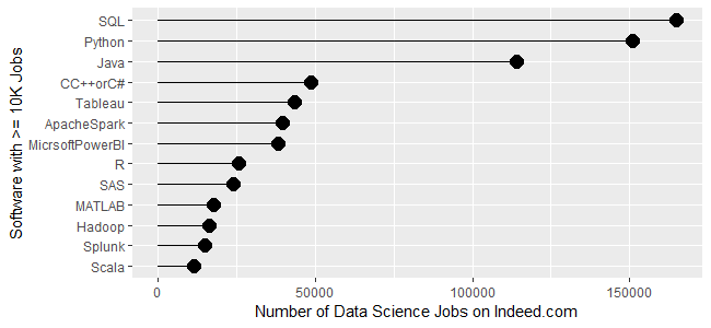
Figure 1a shows the most popular tools, those with at least 10,000 jobs. SQL is in the lead with 164,996 jobs, followed by Python with 150,992 and Java with 113,944. Next comes a set from C++/C# at 48,555, slowly declining to Microsoft’s Power BI at 38,125. Tableau, one of Power BI’s major competitors, is in that set. Next comes R and SAS, both around 24K jobs, with R slightly in the lead. Finally, we see a set slowly declining from MATLAB at 17,736 to Scala at 11,473.
Figure 1a. Number of data science jobs for the more popular software (>= 10,000 jobs).
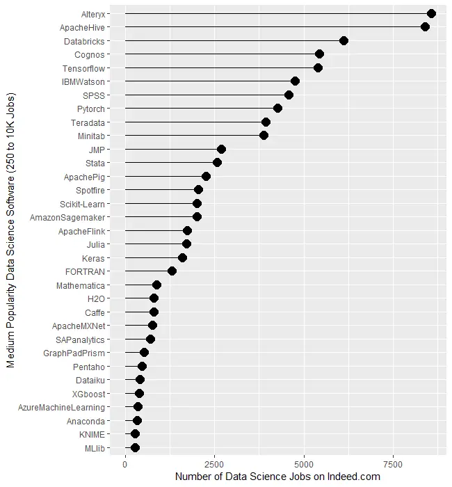
Figure 1b covers tools for which there are between 250 and 10,000 jobs. Alteryx and Apache Hive are at the top, both with around 8,400 jobs. There is quite a jump down to Databricks at 6,117 then much smaller drops from there to Minitab at 3,874. Then we see another big drop down to JMP at 2,693 after which things slowly decline until MLlib at 274.
Figure 1b. Number of jobs for less popular data science software tools, those with between 250 and 10,000 jobs.
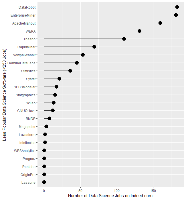
The least popular set of software, those with fewer than 250 jobs, are displayed in Figure 1c. It begins with DataRobot and SAS’ Enterprise Miner, both near 182. That’s followed by Apache Mahout with 160, WEKA with 131, and Theano at 110. From RapidMiner on down, there is a slow decline until we finally hit zero at WPS Analytics. The latter is a version of the SAS language, so advertisements are likely to always list SAS as the required skill.
Figure 1c. Number of jobs for software having fewer than 250 advertisements.
Several tools use the powerful yet easy workflow interface: Alteryx, KNIME, Enterprise Miner, RapidMiner, and SPSS Modeler. The scale of their counts is too broad to make a decent graph, so I have compiled those values in Table 1. There we see Alteryx is extremely dominant, with 30 times as many jobs as its closest competitor, KNIME. The latter is around 50% greater than Enterprise Miner, while RapidMiner and SPSS Modeler are tiny by comparison.
Software
Jobs
Alteryx
8,566
KNIME
281
Enterprise Miner
181
RapidMiner
69
SPSS Modeler
17
Table 1. Job counts for workflow tools.
Let’s take a similar look at packages whose traditional focus was on statistical analysis. They have all added machine learning and artificial intelligence methods, but their reputation still lies mainly in statistics. We saw previously that when we consider the entire range of data science jobs, R was slightly ahead of SAS. Table 2 shows jobs with only the term “statistician” in their description. There we see that SAS comes out on top, though with such a tiny margin over R that you might see the reverse depending on the day you gather new data. Both are over five times as popular as Stata or SPSS, and ten times as popular as JMP. Minitab seems to be the only remaining contender in this arena.
Software
Jobs only for “Statistician”
SAS
1040
R
1012
Stata
176
SPSS
146
JMP
93
Minitab
55
Statistica
2
BMDP
3
Systat
0
NCSS
0
Table 2. Number of jobs for the search term “statistician” and each software.
Next, let’s look at the change in jobs from the 2019 data to now (October 2022), focusing on software that had at least 50 job listings back in 2019. Without such a limitation, software that increased from 1 job in 2019 to 5 jobs in 2022 would have a 500% increase but still would be of little interest. Percent change ranged from -64.0% to 2,479.9%, with a mean of 306.3 and a median of 213.6. There were two extreme outliers, IBM Watson, with apparent job growth of 2,479.9%, and Databricks, at 1,323%. Those two were so much greater than the rest that I left them off of Figure 1d to keep them from compressing the remaining values beyond legibility. The rapid growth of Databricks has been noted elsewhere. However, I would take IBM Watson’s figure with a grain of salt as its growth in revenue seems nowhere near what the Indeed.com’s job figure seems to indicate.
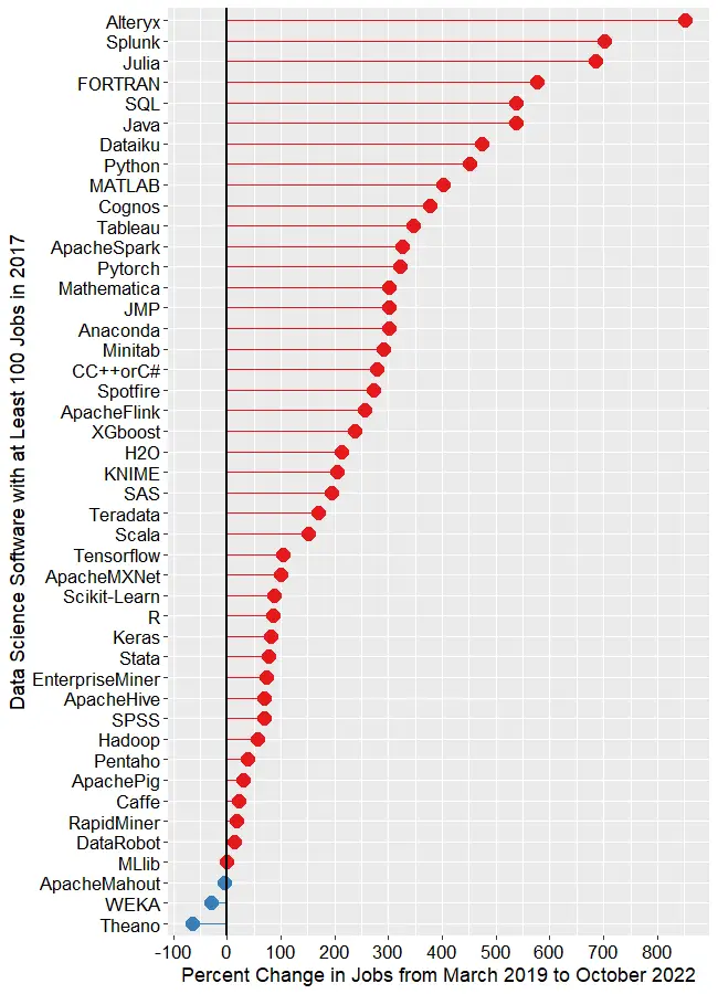
The remaining software is shown in Figure 1d, where those whose job market is “heating up” or growing are shown in red, while those that are cooling down are shown in blue. The main takeaway from this figure is that nearly the entire data science software market has grown over the last 3.5 years. At the top, we see Alteryx, with a growth of 850.7%. Splunk (702.6%) and Julia (686.2%) follow. To my surprise, FORTRAN follows, having gone from 195 jobs to 1,318, yielding growth of 575.9%! My supercomputing colleagues assure me that FORTRAN is still important in their area, but HPC is certainly not growing at that rate. If any readers have ideas on why this could occur, please leave your thoughts in the comments section below.
Figure 1d. Percent change in job listings from March 2019 to October 2022. Only software that had at least 50 jobs in 2019 is shown. IBM (2,480%) and Databricks (1,323%) are excluded to maintain the legibility of the remaining values.
SQL and Java are both growing at around 537%. From Dataiku on down, the rate of growth slows steadily until we reach MLlib, which saw almost no change. Only two packages declined in job advertisements, with WEKA at -29.9%, Theano at -64.1%.
This wraps up my analysis of software popularity based on jobs. You can read my ten other approaches to this task at https://r4stats.com/articles/popularity/. Many of those are based on older data, but I plan to update them in the first quarter of 2023, when much of the needed data will become available. To receive notice of such updates, subscribe to this blog, or follow me on Twitter: https://twitter.com/BobMuenchen.
At the useR! 2022 Conference, the world-renowned Mayo Clinic announced that after 20 years of using SAS Institute’s JMP software, they have migrated to the BlueSky Statistics user interface for R. Ross Dierkhising, a principal biostatistician with the Clinic, described the process. They reviewed 16 commercial statistical software packages and none met their needs as well as JMP. Then they investigated three graphical user interface for the powerful R language: BlueSky Statistics, jamovi, and JASP.
They found BlueSky meet their needs as well as JMP, for significantly less cost. Then Mayo’s staff added over 40 new dialogs to BlueSky, including things that JMP did not offer. Dierkhising said, “I have nothing but the highest respect [for] the BlueSky development team and how they worked with us.” Among others, the Mayo’s additions to BlueSky include:
Kaplan-Meier, one group and compare groups
Competing risks, one group, and compare groups
Cox models, single model, and advanced single model
Stratified cox model
Fine-Gray Cox model
Cox model, with binary time-dependent covariate
Large-scale data/model summaries via the arsenal package
Frequency table in list format
Compare datasets like SAS’ compare procedure
Single tables of multiple model fits
Bland-Altman plots
Cohen’s and Fleiss’ kappa
Concordance correlation coefficients
Intraclass correlation coefficients
Diagnostic testing with a gold standard
Although Dierkhising said BlueSky included a “ton” of data wrangling methods, the Mayo team added a dozen more. The result was “gigantic” cost savings, and a tool that, in the end, did things that JMP could not do.
Anyone can download a free and open source copy of BlueSky statistics from the company website. You can read my detailed review of BlueSky here, and see how it compares to other graphical user interfaces to R here. The BlueSky User Guide is online here.
You can watch Ross Dierkhising’s entire 17 minute presentation here:
I have just updated my detailed reviews of Graphical User Interfaces (GUIs) for R, so let’s compare them again. It’s not too difficult to rank them based on the number of features they offer, so let’s start there. I’m basing the counts on the number of dialog boxes in each category of four categories:
Ease of Use
General Usability
Graphics
Analytics
This is trickier data to collect than you might think. Some software has fewer menu choices, depending instead on more detailed dialog boxes. Studying every menu and dialog box is very time-consuming, but that is what I’ve tried to do. I’m putting the details of each measure in the appendix so you can adjust the figures and create your own categories. If you decide to make your own graphs, I’d love to hear from you in the comments below.
Figure 1 shows how the various GUIs compare on the average rank of the four categories. R Commander is abbreviated Rcmdr, and R AnalyticFlow is abbreviated RAF. We see that BlueSky is in the lead with R-Instat close behind. As my detailed reviews of those two point out, they are extremely different pieces of software! Rather than spend more time on this summary plot, let’s examine the four categories separately.
Figure 1. Mean of each R GUI’s ranking of the four categories. To make this plot consistent with the others below, the larger the rank, the better.
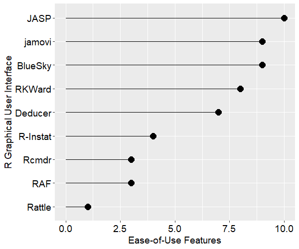
For the category of ease-of-use, I’ve defined it mostly by how well each GUI does what GUI users are looking for: avoiding code. They get one point each for being able to install, start, and use the GUI to its maximum effect, including publication-quality output, without knowing anything about the R language itself. Figure two shows the result. JASP comes out on top here, with jamovi and BlueSky right behind.
Figure 2. The number of ease-of-use features that each GUI has.
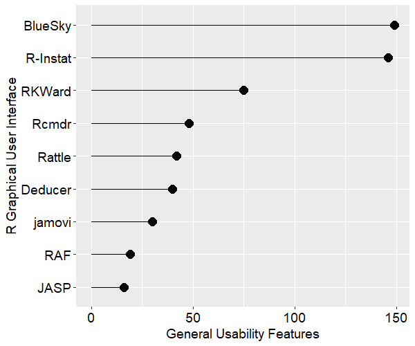
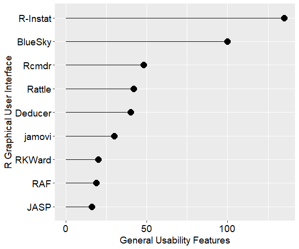
Figure 3 shows the general usability features each GUI offers. This category is dominated by data-wrangling capabilities, where data scientists and statisticians spend most of their time. This category also includes various types of data input and output. BlueSky and R-Instat come out on top not just due to their excellent selection of data wrangling features but also due to their use of the rio package for importing and exporting files. The rio package combines the import/export capabilities of many other packages, and it is easy to use. I expect the other GUIs will eventually adopt it, raising their scores by around 40 points. JASP shows up at the bottom of this plot due to its philosophy of encouraging users to prepare the data elsewhere before importing it into JASP.
Figure 3. Number of general usability features for each GUI.
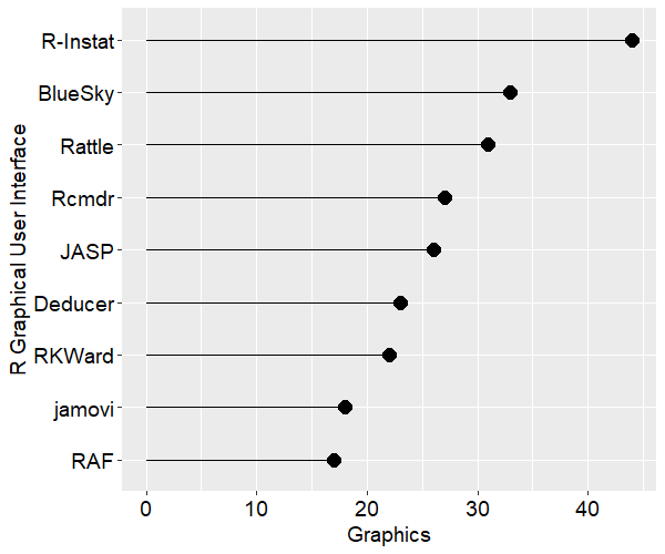
Figure 4 shows the number of graphics features offered by each GUI. R-Instat has a solid lead in this category. In fact, this underestimates R-Instat’s ability if you…
I have recently updated my detailed reviews of Graphical User Interfaces (GUIs) for R, so it’s time for another comparison post. It’s not too difficult to rank them based on the number of features they offer, so let’s start there. I’m basing the counts on the number of dialog boxes in each category of four categories:
Ease of Use
General Usability
Graphics
Analytics
This is trickier data to collect than you might think. Some software has fewer menu choices, depending instead on more detailed dialog boxes. Studying every menu and dialog box is very time-consuming, but that is what I’ve tried to do. I’m putting the details of each measure in the appendix so you can adjust the figures and create your own categories. If you decide to make your own graphs, I’d love to hear from you in the comments below.
Figure 1 shows how the various GUIs compare on the average rank of the four categories. R Commander is abbreviated Rcmdr, and R AnalyticFlow is abbreviated RAF. We see that BlueSky (User Guide online here) and R-Instat are nearly tied for the lead. As my detailed reviews of those two point out, they are extremely different pieces of software! Rather than spend more time on this summary plot, let’s examine the four categories separately.
Figure 1. Mean of each R GUI’s ranking of the four categories. To make this plot consistent with the others below, the larger the rank, the better.
For the category of ease-of-use, I’ve defined it mostly by how well each GUI does what GUI users are looking for: avoiding code. They get one point each for being able to install, start, and use the GUI to its maximum effect, including publication-quality output without having to know anything about the R language itself. Figure two shows the result. JASP comes out on top here, with jamovi and BlueSky right behind.
Figure 2. The number of ease-of-use features that each GUI has.
Figure 3 shows the general usability features each GUI offers. This category is dominated by data-wrangling capabilities, where data scientists and statisticians spend the majority of their time. This category also includes various types of data input and output. R-Instat comes out on top not just due to its excellent selection of data wrangling features, but also due to its use of the rio package for importing and exporting files. The rio package combines the import/export capabilities of many other packages and it is easy to use. I expect the other GUIs will eventually adopt it, raising their scores by around 40 points. JASP shows up at the bottom on this plot due to its philosophy of encouraging users to prepare the data elsewhere before importing it into JASP.
Figure 3. Number of general usability features for each GUI.
Figure 4 shows the number of graphics features offered by each GUI. R-Instat has a solid lead in this category. In fact, this is actually an underestimate of R-Instat’s ability if you include its options to layer any “geom” on top of any graph. However, that requires knowing what the geoms are and how to use them. That’s knowledge of R code, of course.
When studying these graphs, it’s important to consider the difference between the relative and absolute performance. For example, relatively speaking, JASP and R Commander are not doing well here, but they do offer over 25 types of plots! That absolute figure might be fine for your needs.
Figure 4. Number of graphics features offered by each GUI.
Finally, we get to what is, for many people, the main reason for using this type of software: analytics. Figure 5 shows how the GUIs compare on the number of statistics, machine learning, and artificial intelligence methods. Here R Commander shows, well, a “commanding” lead! This GUI has been around the longest, and so has had more time for people to contribute to its capabilities. If you read an earlier version of this article, R Commander was not as dominant. That was due to the fact that I had not yet taken the time necessary to load and study every one of its 42 add-ons. That required a substantial amount of time, and these updated figures reflect a more complete view of its capabilities.
Again, it’s worth considering the absolute values on the x-axis. JASP and jamovi are in the middle of the pack, but they both have nearly 200 methods. If that is sufficient for your needs, you can then focus on the other categories.
Many important details are buried in these simple counts. For example, I enjoy using jamovi for statistical analyses, but it currently lacks machine learning and artificial intelligence. I like BlueSky too, but it doesn’t yet do any Bayesian statistics (jamovi and JASP do). Rattle comes out near the bottom due to its focus on machine learning, but it does an excellent job of introducing students to that area.
Figure 5. Number of analytics features offered by each GUI.
Overview of Each R GUI
The above plots help show us overall feature sets, but each package offers methods that the others lack. Let’s look at a brief overview of each. Remember that each of these has a detailed review that follows my standard template. I present them in alphabetical order.
BlueSky Statistics – This software was created by former SPSS employees and it shares many of SPSS’ features. BlueSky is only a few years old, and it converted from commercial to open source mid-way through 2018. Its developers have been adding features at a rapid rate. When using BlueSky, it’s not initially apparent that R is involved at all. Unless you click the code button “</>” included in every dialog box, you’ll never see the R code. If you’re wanting to learn R code, seeing what BlueSky uses for each step can help. BlueSky saves the dialog settings for every step, providing GUI-based reproducibility. For R code, it uses the popular, but controversial, tidyverse style while most of the other GUIs use base R functions. BlueSky’s output is in publication-quality tables which follow the popular style of the American Psychological Association. It’s stronger than most of the others at AI/ML and psychometrics. It is now available for Windows and Mac (previous versions were Windows-only).
Deducer – This has a very nice-looking interface, and it’s probably the first R GUI to offer output in true APA-style word processing tables. Being able to just cut and paste a table into your word processor saves a lot of time and it’s a feature that has been copied by several others. Deducer was released in 2008, and when I first saw it, I thought it would quickly gain developers. It got a few, but development seems to have halted. Deducer’s installation is quite complex, and it depends on the troublesome Java software. It also uses JGR, which never became as popular as the similar RStudio. The main developer, Ian Fellows, has moved on to another interesting GUI project called Vivid. I ran this most recently in February, 2022, and the output had many odd characters in it, perhaps due to a lack of support for Unicode.
jamovi– The developers who form the core of the jamovi project used to be part of the JASP team. Despite the fact that they started a couple of years later, they’re ahead of JASP in several ways at the moment. Its developers decided that the R code it used should be visible and any R code should be executable, features that differentiated it from JASP. jamovi has an extremely interactive interface that shows you the result of every selection in each dialog box (JASP does too). It also saves the settings in every dialog box, and lets you re-use every step on a new dataset by saving a “template.” That’s extremely useful since GUI users often prefer to avoid learning R code. jamovi’s biggest weakness is its dearth of data management featues, though there are plans to address that. The most recent version of jamovi borrowed the Bayesian analysis methods from JASP, making those two tied as the leaders in that approach. jamovi can help you learn R code by showing what it does at each step, though it uses its own functions from the jmv package. While those functions are not standard R, they do combine the capability of many R functions in each one.
JASP– The biggest advantage JASP offers is its emphasis on Bayesian analysis. If that’s your preference, this might be the one for you. Another strength is JASP’s Machine Learning module. At the moment JASP is very different from all the other GUIs reviewed here because it can’t show you the R code it’s writing. The development team plans to address that issue, but it has been planned for a couple of years now, so it must not be an easy thing to add.
R AnalyticFlow – This is unique among R GUIs as it is the only one that lets you organize your analyses using flowchart-like workflow diagrams. That approach makes it easy to visualize what a complex analysis is doing and to rerun it. It writes very clean base R code and provides easy access to the powerful lattice graphics package. It also supports the ggplot2 graphics package, but only through its more limited quickplot function. R AnalyticFlow also lets you extend its capability making it easier for R power users to interact with non-programmers. However, it has some serious limitations. Its set of analytic and graphical methods is quite sparse. It also lacks the important advantage that most workflow-based tools have: the ability to re-use the workflow on a new dataset by changing only the data input nodes. Since each node requires the name of the dataset used, you must change it in each location.
Rattle– If your work involves ML/AI (a.k.a. data mining) instead of standard statistical methods, Rattle may be the GUI for you. It’s focused on ML/AI, and its tabbed-based interface makes quick work of it. However, it’s the weakest of them all when it comes to statistical analysis. It also lacks many standard data management features.
R Commander – This is the oldest GUI, having been around since at least 2005. There are an impressive 42 add-ons developed for it. It is currently one of only three R GUIs that saves R Markdown files (the others being BlueSky and RKWard), but it does not create word processing tables by default, as some of the others do. The R code it writes is classic, rarely using the newer tidyverse functions. It works as a partner to R; you install R separately, then use it to install and start R Commander. R Commander makes it easy to blend menu-based analysis with coding. If your goal is to learn to code using base R, this is an excellent choice. The software’s main developer, John Fox, told me in January 2022 that he has no future development plans for R Commander. However, others can still extend its feature set by writing add-ons.
R-Instat – This offers one of the most extensive collections of data wrangling, graphics, and statistical analysis methods of any R GUI. At a basic level, its graphics dialogs are easy to use, and it offers powerful multi-layer support for people who are familiar with the ggplot2 package’s geom functions. To use its full modeling capabilities, you need to know what R’s packages (e.g. MASS) are and what each one’s functions (e.g. rlm) do. For an R programmer, recognizing a known package::function combination is much easier than recalling it without assistance. Such a user would find R-Instat’s GUI extremely helpful.
RKWard– This GUI blends a nice point-and-click interface with an integrated development environment (IDE) that is the most advanced of all the other GUIs reviewed here. It’s easy to install and start, and it saves all your dialog box settings, allowing you to rerun them. However, that’s done step-by-step, not all at once as jamovi’s templates allow. The code RKWard creates is classic R, with no tidyverse at all. RKWard is one of only three R GUIs that supports R Markdown.
Conclusion
I hope this brief comparison will help you choose the R GUI that is right for you. Each offers unique features that can make life easier for non-programmers. Instructors of introductory classes in statistics or ML/AI should find these enable their students to focus on the material rather than on learning the R language. If one catches your eye, don’t forget to read the full review of it here.
Acknowledgements
Writing this set of reviews has been a monumental undertaking. It would not have been possible without the assistance of Bruno Boutin, Anil Dabral, Ian Fellows, John Fox, Thomas Friedrichsmeier, Rachel Ladd, Jonathan Love, Ruben Ortiz, Danny Parsons, Christina Peterson, Josh Price, David Stern, Roger Stern, and Eric-Jan Wagenmakers, and Graham Williams.
Appendix: Guide to Scoring
The four categories are defined by the following. The yes/no items get scored 1 for yes, and 0 for no. The “how many” items consist of simple unweighted counts of the number of features, e.g., the number of file types a package can import without relying on R code. I used to plot the total number of features, but that is now dominated by the large values for analytics features, making that total fairly redundant.
Category
Feature
BlueSky
Deducer
Jasp
jamovi
RAF
Rattle
Rcmdr
R-Instat
RKWard
Ease_of_Use
Installs without the use of R
1.00
0.00
1.00
1.00
0.00
0.00
0.00
1.00
1.00
Ease_of_Use
Starts without the use of R
1.00
1.00
1.00
1.00
1.00
0.00
0.00
1.00
1.00
Ease_of_Use
Remembers recent files
0.00
1.00
1.00
1.00
1.00
0.00
0.00
1.00
1.00
Ease_of_Use
Hides R code by default
1.00
1.00
1.00
1.00
0.00
0.00
0.00
0.00
1.00
Ease_of_Use
Use its full capability without using R
1.00
1.00
1.00
1.00
0.00
1.00
1.00
0.00
1.00
Ease_of_Use
Data Editor
1.00
1.00
0.00
1.00
1.00
0.00
1.00
1.00
1.00
Ease_of_Use
Reuse the entire workflow without using R
1.00
0.00
1.00
1.00
0.00
0.00
0.00
0.00
1.00
Ease_of_Use
Pub-quality tables w/out R code steps
1.00
1.00
1.00
1.00
0.00
0.00
0.00
0.00
0.00
Ease_of_Use
Hides field-specific menus initially
0.00
1.00
1.00
1.00
0.00
0.00
1.00
0.00
0.00
Ease_of_Use
Table of Contents to ease navigation
0.00
0.00
1.00
0.00
0.00
0.00
0.00
0.00
1.00
Ease_of_Use
Easy to move blocks of output
1.00
0.00
1.00
0.00
0.00
0.00
0.00
0.00
0.00
Ease_of_Use
Easy to repeat any step by groups
1.00
0.00
0.00
0.00
0.00
0.00
0.00
0.00
0.00
General_Features
Operating Systems (how many)
2.00
3.00
4.00
4.00
3.00
3.00
3.00
1.00
3.00
General_Features
Import Data File Types (how many)
7.00
15.00
6.00
6.00
1.00
9.00
7.00
31.00
5.00
General_Features
Import Database (how many)
5.00
0.00
0.00
0.00
0.00
1.00
0.00
1.00
0.00
General_Features
Export Data File Types (how many)
5.00
7.00
1.00
5.00
1.00
1.00
3.00
20.00
3.00
General_Features
Multiple Data Files Open at Once
1.00
1.00
0.00
0.00
0.00
0.00
0.00
1.00
0.00
General_Features
Multiple Output Windows
1.00
0.00
0.00
0.00
0.00
0.00
0.00
0.00
0.00
General_Features
Multiple Code Windows
0.00
0.00
0.00
0.00
0.00
0.00
0.00
0.00
0.00
General_Features
Variable Metadata View
1.00
1.00
0.00
1.00
0.00
0.00
0.00
1.00
1.00
General_Features
Variable Search in Dialogs
0.00
1.00
0.00
1.00
0.00
0.00
0.00
0.00
0.00
General_Features
Variable Filtering (limit vars shown in data and dialogs)
R-Instat is a free and open source graphical user interface for the R software that focuses on people who want to point-and-click their way through data science analyses. Written in Visual Basic, it is currently only available for Microsoft Windows. However, a Linux version is in development using the cross-platform Mono implementation of the .NET framework.This post is one of a series of reviews that aim to help non-programmers choose the Graphical User Interface (GUI) that is best for them. Although I wrote the BlueSky User’s Guide, I hope to remain objective in these reviews. There is no one perfect user interface for everyone; each GUI for R has features that appeal to a different set of people.
Terminology
There are various definitions of user interface types, so here’s how I’ll be using these terms:GUI = Graphical User Interface using menus and dialog boxes to avoid having to type programming code. I do not include any assistance for programming in this definition. So, GUI users are people who prefer using a GUI to perform their analyses. They don’t have the time or inclination to become good programmers.
IDE = Integrated Development Environment which helps programmers write code. I do not include point-and-click style menus and dialog boxes when using this term. IDE users are people who prefer to write R code to perform their analyses.
Installation
The various user interfaces available for R differ quite a lot in how they’re installed. Some, such as jamovi or RKWard, install in a single step. Others, such as Deducer, install in multiple steps (up to seven steps, depending on your needs). Advanced computer users often don’t appreciate how lost beginners can become while attempting even a simple installation. The HelpDesks at most universities are flooded with such calls at the beginning of each semester!
R-Instat is easy to install, requiring only a single step. It provides its own embedded copy of R. This simplifies the installation and ensures complete compatibility between R-Instat and the version of R it’s using. However, it also means if you already have R installed, you’ll end up with a second copy. You can have R-Instat control any version of R you choose, but if the version differs too much, you may run into occasional problems.
Plug-in Modules
When choosing a GUI, one of the most fundamental questions is: what can it do for you? What the initial software installation of each GUI gets you is covered in the Graphics, Analysis, and Modeling sections of this series of articles. Regardless of what comes built-in, it’s good to know how active the development community is. They contribute “plug-ins” that add new menus and dialog boxes to the GUI. This level of activity ranges from very low (RKWard, Rattle, Deducer) through medium (JASP 15) to high (jamovi 43, R Commander 43).
While the R-Instat project welcomes contributions from anyone, there are not any modules to add at this time. All of its capabilities are included in its initial installation.
Startup
Some user interfaces for R, such as jamovi or JASP, start by double-clicking on a single icon, which is great for people who prefer to not write code. Others, such as R commander and JGR, have you start R, then load a package from your library, and then finally call a function. That’s better for people looking to learn R, as those are among the first tasks they’ll have to learn anyway.
You start R-Instat directly by double-clicking its icon from your desktop or choosing it from your Start Menu (i.e., not from within R).
Data Editor
A data editor is a fundamental feature in data analysis software. It puts you in touch with your data and lets you get a feel for it, if only in a rough way. A data editor is such a simple concept that you might think there would be hardly any differences in how they work in different GUIs. While there are technical differences, to a beginner what matters the most are the differences in simplicity. Some GUIs, including jamovi, let you create only what R calls a data frame. They use more common terminology and call it a data set: you create one, you save one, later you open one, then you use one. Others, such as RKWard trade this simplicity for the full R language perspective: a data set is stored in a workspace. So the process goes: you create a data set, you save a workspace, you open a workspace, and choose a data set from within it.
R-Instat starts up by showing its screen (Fig. 1). Under Start, I chose “New Data Frame” and it showed me the rather perplexing dialog shown in Fig. 2.
Figure 1. The R-Instat startup screen.
As an R user, I know what expressions are, but what did the R-Instat designers mean by the term?
Figure 2. The New Dataframe dialog.
Clicking the “Construct Examples” button brought up the suggestions shown in Fig. 3. These are standard R expressions, which came as quite a surprise! It seems that the R-Instat designers are wanting to get people to start using R programming code immediately.
Figure 3. Examples R-Instat provides for expression you can use to create a dataset.
Clicking the Help button brings up the advice, “the simplest option is Empty” (the developers say this will become the default in a future version). Clicking that button brings up a simple prompt for the number of rows and columns you would like to create. After that, you’re looking at a basic spreadsheet (Fig. 4) that easily lets you enter data. As you enter data, it determines if it is numeric or character. Scientific notation is accepted, but dates are saved as character variables. Logical values (TRUE, FALSE) are recognized as such and are stored appropriately.
Right-clicking on any column allows you to convert variables to be a factor, ordered factor, numeric, logical, or character. These changes are recorded as function calls to a custom “convert_column_to_type” function for reproducibility. Such interactive changes are not usually recorded by other R GUIs. Date/time conversion is not available on that menu, as that process is trickier. Those conversions are on the “Prepare> Column Date” menu item. Other things you can do from the right-click menu are: rename, duplicate, reorder, set levels/labels, sort, and filter/remove filter.
The class of each variable is indicated by a character code that follows each variable name in parenthesis: (C) for character, (F) for factor, (O.F) for ordered factor, (D) for date, (L) for logical. When no code follows a variable name, it is numeric.
Figure 4. The R-Instat Data View (left) and Output Window (right).
The name of the dataset appears on a tab at the bottom of the Data View window. This lets you easily manage multiple datasets, an ability that is popular among professionals, but which is rarely offered in R GUIs (BlueSky and R Commander are the only others that offer it).
Once the dataset is saved, to add rows or columns you choose, “Prepare > Data Frame > Insert rows/columns” to add new rows or columns at any position in the data frame. New columns can be added with a specified default value, which can be a big time-saver when entering blocks of related data.
There is a quicker method that works for inserting new rows. You right-click the row numbers and a pop-up menu will allow you to insert rows above or below, and the number of rows selected is the number of rows added – like in Excel.
When editing data, R-Instat lets you type new values on top of the old. As soon as you press the Enter key, it generates R code to execute the change. For example, in a language variable, when changing the value “English” to “Spanish,” it wrote,
Replace Value in Data
data_book$replace_value_in_data(data_name="wakefield", col_name="Language", rows="78", new_value="Spanish")
This is important for reproducibility, but R-Instat is the only GUI reviewed here that tracks such important manual changes. In fact, even among expensive proprietary software, Stata is the only one that I’m aware of that keeps track of such changes using code.
If you have another data set to enter, you can restart the process by choosing “File> New Data…” again. You can change data sets simply by clicking on its tab, and its window will pop to the front for you to see. When doing analyses, or saving data, the data set that is displayed in the editor does not influence what appears in dialog boxes. That means that you can be looking at one dataset while analyzing another! Since each dialog allows you to choose the dataset to use, that is technically not a problem, but if you have several datasets that contain the same variable names, remember that what you see may not be what you get! That’s the opposite of BlueSky Statistics, which automatically analyzes the dataset you see. R-Instat’s ability to work with multiple datasets in a single instance of the software is not a feature found in all R GUIs. For example, jamovi and JASP can only work with a single dataset at a time.
Saving the data is done with a fairly standard “File> Save As> Save Dataset As” menu. By default it will save all open datasets, filters, graphs, and models to a single file called a “data book.” That makes working with complex projects much easier to open and close.
Data Import
R-Instat supports the following file formats, most of which are automatically opened using “File> Import from File”. The ODK and NetCDF file formats have their own Import menus. R-Instat’s ability to open many formats related to climate science hints at what the software excels at. For details, see the Analysis Methods section below.
Comma Separated Values (.csv)
Plain text files (.txt)
Excel (old and new xls file types)
xBASE database files (dBase, etc.)
SPSS (.sav)
SAS binary files (sas7bdat and *.xpt)
Standard R workspace files (RData, but it just opens one dataframe of its choosing)
BlueSky Statistics is an easy-to-use menu system that uses the R language to do all its work. My detailed review of BlueSky is available here, and a brief comparison of the various menu systems for R is here. I’ve just released the BlueSky Statistics 7.1 User Guide in printed form on the world’s largest independent bookstore, Lulu.com. A description and detailed table of contents are available here.
Cover design by Kiran Rafiq.
I’ve also released the BlueSky Statistics 7.1 Intro Guide. It is a complete subset of the User Guide, and you can download it for free here (if you have trouble downloading it, your company may have security blocking Microsoft OneDrive; try it at home). Its description and table of contents are here, and soon you will also be able to purchase a printed copy of it from Lulu.com.
Cover design by Kiran Rafiq.
I’m enthusiastic about getting feedback on these books. If you have comments or suggestions, please send them to me at muenchen.bob at gmail dot com.
Publishing with Lulu.com has been a very pleasant experience. They put the author in complete control, making one responsible for every detail of the contents, obtaining reviewers, creating a cover file that includes the front, back, and spine of the book to match the dimensions of the book (e.g. more pages means wider spine, etc.) Advertising is left up to the writer as well, hence this blog post! If you are thinking about writing a book, I highly recommend both Lulu.com and getting a cover design from 99designs.com. The latter let me run a contest in which a dozen artists submitted several ideas each. Their built-in survey system let me ask many colleagues for their opinions to help me decide. Altogether, it was a very interesting experience.
To follow the progress of these and other R related books, subscribe to my blog, or follow me on Twitter.
The BlueSky Statistics graphical user interface (GUI) for the R language has added quite a few new features (described below). I’m also working on a BlueSky User Guide, a draft of which you can read about and download here. [Update: don’t download that, get the full Intro Guide download instead.] Although I’m spending a lot of time on BlueSky, I still plan to be as obsessive as ever about reviewing all (or nearly all) of the R GUIs, which is summarized here.
The new data management features in BlueSky are:
Date Order Check — this lets you quickly check across the dates stored in many variables, and it reports if it finds any rows whose dates are not always increasing from left to right.
Find Duplicates – generates a report of duplicates and saves a copy of the data set from which the duplicates are removed. Duplicates can be based on all variables, or a set of just ID variables.
Select First/Last Observation per Group – finding the first or last observation in a group can create new datasets from the “best” or “worst” case in each group, find the most current record, and so on.
Model Fitting / Tuning
One of the more interesting features in BlueSky is its offering of what they call Model Fitting and Model Tuning. Model Fitting gives you direct control over the R function that does the work. That provides precise control over every setting, and it can teach you the code that the menus create, but it also means that model tuning is up to you to do. However, it does standardize scoring so that you do not have to keep up with the wide range of parameters that each of those functions need for scoring. Model Tuning controls models through the caret package, which lets you do things like K-fold cross-validation and model tuning. However, it does not allow control over every model setting.
New Model Fitting menu items are:
Cox Proportional Hazards Model: Cox Single Model
Cox Multiple Models
Cox with Formula
Cox Stratified Model
Extreme Gradient Boosting
KNN
Mixed Models
Neural Nets: Multi-layer Perceptron
NeuralNets (i.e. the package of that name)
Quantile Regression
There are so many Model Tuning entries that it’s easier to just paste in the list I updated on the main BlueSkly review that I updated earlier this morning:
Model Tuning: Adaboost Classification Trees
Model Tuning: Bagged Logic Regression
Model Tuning: Bayesian Ridge Regression
Model Tuning: Boosted trees: gbm
Model Tuning: Boosted trees: xgbtree
Model Tuning: Boosted trees: C5.0
Model Tuning: Bootstrap Resample
Model Tuning: Decision trees: C5.0tree
Model Tuning: Decision trees: ctree
Model Tuning: Decision trees: rpart (CART)
Model Tuning: K-fold Cross-Validation
Model Tuning: K Nearest Neighbors
Model Tuning: Leave One Out Cross-Validation
Model Tuning: Linear Regression: lm
Model Tuning: Linear Regression: lmStepAIC
Model Tuning: Logistic Regression: glm
Model Tuning: Logistic Regression: glmnet
Model Tuning: Multi-variate Adaptive Regression Splines (MARS via earth package)
Model Tuning: Naive Bayes
Model Tuning: Neural Network: nnet
Model Tuning: Neural Network: neuralnet
Model Tuning: Neural Network: dnn (Deep Neural Net)
Model Tuning: Neural Network: rbf
Model Tuning: Neural Network: mlp
Model Tuning: Random Forest: rf
Model Tuning: Random Forest: cforest (uses ctree algorithm)