The Tidyverse Curse

I’ve just finished a major overhaul to my widely read article, Why R is Hard to Learn. It describes the main complaints I’ve heard from the participants to my workshops, and how those complaints can often be mitigated. Here’s the only new section:

The Tidyverse Curse

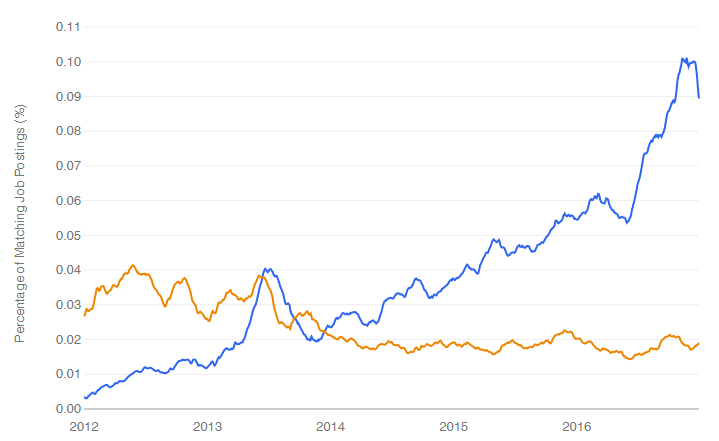
There’s a common theme in many of the sections above: a task that is hard to perform using base a R function is made much easier by a function in the dplyr package. That package, and its relatives, are collectively known as the tidyverse. Its functions help with many tasks, such as selecting, renaming, or transforming variables, filtering or sorting observations, combining data frames, and doing by-group analyses. dplyr is such a helpful package that Rdocumentation.org shows that it is the single most popular R package (as of 3/23/2017.) As much of a blessing as these commands are, they’re also a curse to beginners as they’re more to learn. The main packages of dplyr, tibble, tidyr, and purrr contain a few hundred functions, though I use “only” around 60 of them regularly. As people learn R, they often comment that base R functions and tidyverse ones feel like two separate languages. The tidyverse functions are often the easiest to use, but not always; its pipe operator is usually simpler to use, but not always; tibbles are usually accepted by non-tidyverse functions, but not always; grouped tibbles may help do what you want automatically, but not always (i.e. you may need to ungroup or group_by higher levels). Navigating the balance between base R and the tidyverse is a challenge to learn.

A demonstration of the mental overhead required to use tidyverse function involves the usually simple process of printing data. I mentioned this briefly in the Identity Crisis section above. Let’s look at an example using the built-in mtcars data set using R’s built-in print function:

> print(mtcars)
                  mpg cyl disp  hp drat    wt  qsec vs am gear carb
Mazda RX4         21.0 6 160.0 110 3.90 2.620 16.46  0  1    4    4
Mazda RX4 Wag     21.0 6 160.0 110 3.90 2.875 17.02  0  1    4    4
Datsun 710        22.8 4 108.0  93 3.85 2.320 18.61  1  1    4    1
Hornet 4 Drive    21.4 6 258.0 110 3.08 3.215 19.44  1  0    3    1
Hornet Sportabout 18.7 8 360.0 175 3.15 3.440 17.02  0  0    3    2
Valiant           18.1 6 225.0 105 2.76 3.460 20.22  1  0    3    1
...

We see the data, but the variable names actually ran off the top of my screen when viewing the entire data set, so I had to scroll backwards to see what they were. The dplyr package adds several nice new features to the print function. Below, I’m taking mtcars and sending it using the pipe operator “%>%” into dplyr’s as_data_frame function to convert it to a special type of tidyverse data frame called a “tibble” which prints better. From there I send it to the print function (that’s R’s default function, so I could have skipped that step). The output all fits on one screen since it stopped at a default of 10 observations. That allowed me to easily see the variable names that had scrolled off the screen using R’s default print method.  It also notes helpfully that there are 22 more rows in the data that are not shown. Additional information includes the row and column counts at the top (32 x 11), and the fact that the variables are stored in double precision (<dbl>).

> library("dplyr")
> mtcars %>%
+   as_data_frame() %>%
+   print()
# A tibble: 32 × 11
   mpg   cyl  disp    hp  drat    wt  qsec    vs   am   gear  carb
* <dbl> <dbl> <dbl> <dbl> <dbl> <dbl> <dbl> <dbl> <dbl> <dbl> <dbl>
 1 21.0   6   160.0  110  3.90 2.620 16.46    0     1     4     4
 2 21.0   6   160.0  110  3.90 2.875 17.02    0     1     4     4
 3 22.8   4   108.0   93  3.85 2.320 18.61    1     1     4     1
 4 21.4   6   258.0  110  3.08 3.215 19.44    1     0     3     1
 5 18.7   8   360.0  175  3.15 3.440 17.02    0     0     3     2
 6 18.1   6   225.0  105  2.76 3.460 20.22    1     0     3     1
 7 14.3   8   360.0  245  3.21 3.570 15.84    0     0     3     4
 8 24.4   4   146.7   62  3.69 3.190 20.00    1     0     4     2
 9 22.8   4   140.8   95  3.92 3.150 22.90    1     0     4     2
10 19.2   6   167.6  123  3.92 3.440 18.30    1     0     4     4
# ... with 22 more rows

The new print format is helpful, but we also lost something important: the names of the cars! It turns out that row names get in the way of the data wrangling that dplyr is so good at, so tidyverse functions replace row names with 1, 2, 3…. However, the names are still available if you use the rownames_to_columns() function:

> library("dplyr")
> mtcars %>%
+   as_data_frame() %>%
+   rownames_to_column() %>%
+   print()
Error in function_list[[i]](value) : 
 could not find function "rownames_to_column"

Oops, I got an error message; the function wasn’t found. I remembered the right command, and using the dplyr package did cause the car names to vanish, but the solution is in the tibble package that I “forgot” to load. So let’s load that too (dplyr is already loaded, but I’m listing it again here just to make each example stand alone.)

> library("dplyr")
> library("tibble")
> mtcars %>%
+   as_data_frame() %>%
+   rownames_to_column() %>%
+   print()
# A tibble: 32 × 12
 rowname            mpg   cyl disp    hp   drat   wt   qsec   vs    am   gear carb
  <chr>            <dbl> <dbl> <dbl> <dbl> <dbl> <dbl> <dbl> <dbl> <dbl> <dbl> <dbl>
1 Mazda RX4         21.0   6   160.0  110  3.90  2.620 16.46   0     1     4     4
2 Mazda RX4 Wag     21.0   6   160.0  110  3.90  2.875 17.02   0     1     4     4
3 Datsun 710        22.8   4   108.0   93  3.85  2.320 18.61   1     1     4     1
4 Hornet 4 Drive    21.4   6   258.0  110  3.08  3.215 19.44   1     0     3     1
5 Hornet Sportabout 18.7   8   360.0  175  3.15  3.440 17.02   0     0     3     2
6 Valiant           18.1   6   225.0  105  2.76  3.460 20.22   1     0     3     1
7 Duster 360        14.3   8   360.0  245  3.21  3.570 15.84   0     0     3     4
8 Merc 240D         24.4   4   146.7   62  3.69  3.190 20.00   1     0     4     2
9 Merc 230          22.8   4   140.8   95  3.92  3.150 22.90   1     0     4     2
10 Merc 280         19.2   6   167.6  123  3.92  3.440 18.30   1     0     4     4
# ... with 22 more rows

Another way I could have avoided that problem is by loading the package named tidyverse, which includes both dplyr and tibble, but that’s another detail to learn.

In the above output, the row names are back! What if we now decided to save the data for use with a function that would automatically display row names? It would not find them because now they’re now stored in a variable called rowname, not in the row names position! Therefore, we would need to use either the built-in names function or the tibble package’s column_to_rownames function to restore the names to their previous position.

Most other data science software requires row names to be stored in a standard variable e.g. rowname. You then supply its name to procedures with something like SAS’
“ID rowname;” statement. That’s less to learn.

This isn’t a defect of the tidyverse, it’s the result of an architectural decision on the part of the original language designers; it probably seemed like a good idea at the time. The tidyverse functions are just doing the best they can with the existing architecture.

Another example of the difference between base R and the tidyverse can be seen when dealing with long text strings. Here I have a data frame in tidyverse format (a tibble). I’m asking it to print the lyrics for the song American Pie. Tibbles normally print in a nicer format than standard R data frames, but for long strings, they only display what fits on a single line:

> songs_df %>%
+   filter(song == "american pie") %>%
+   select(lyrics) %>%
+   print()
# A tibble: 1 × 1
 lyrics
 <chr>
1 a long long time ago i can still remember how that music used

The whole song can be displayed by converting the tibble to a standard R data frame by routing it through the as.data.frame function:

> songs_df %>%
+   filter(song == "american pie") %>%
+   select(lyrics) %>%
+   as.data.frame() %>%
+   print()
 ... <truncated>
1 a long long time ago i can still remember how that music used 
to make me smile and i knew if i had my chance that i could make 
those people dance and maybe theyd be happy for a while but 
february made me shiver with every paper id deliver bad news on 
the doorstep i couldnt take one more step i cant remember if i cried 
...

These examples demonstrate a small slice of the mental overhead you’ll need to deal with as you learn base R and the tidyverse packages, such as dplyr. Since this section has focused on what makes R hard to learn, it may make you wonder why dplyr is the most popular R package. You can get a feel for that by reading the Introduction to dplyr. Putting in the time to learn it is well worth the effort.

Forrester’s 2017 Take on Tools for Data Science

In my ongoing quest to track The Popularity of Data Science Software, I’ve updated the discussion of the annual report from Forrester, which I repeat here to save you from having to read through the entire document. If your organization is looking for training in the R language, you might consider my books, R for SAS and SPSS Users or R for Stata Users, or my on-site workshops.

Forrester Research, Inc. is a company that provides reports which analyze the competitive position of tools for data science. The conclusions from their 2017 report, Forrester Wave: Predictive Analytics and Machine Learning Solutions, are summarized in Figure 3b. On the x-axis they list the strength of each company’s strategy, while the y-axis measures the strength of their current offering. The size and shading of the circles around each data point indicate the strength of each vendor in the marketplace (70% vendor size, 30% ISV and service partners).

As with Gartner 2017 report discussed above, IBM, SAS, KNIME, and RapidMiner are considered leaders. However, Forrester sees several more companies in this category: Angoss, FICO, and SAP. This is quite different from the Gartner analysis, which places Angoss and SAP in the middle of the pack, while FICO is considered a niche player.

Figure 3b. Forrester Wave plot of predictive analytics and machine learning software.

In their Strong Performers category, they have H2O.ai, Microsoft, Statistica, Alpine Data, Dataiku, and, just barely, Domino Data Labs. Gartner rates Dataiku quite a bit higher, but they generally agree on the others. The exception is that Gartner dropped coverage of Alpine Data in 2017. Finally, Salford Systems is in the Contenders section. Salford was recently purchased by Minitab, a company that has never been rated by either Gartner or Forrester before as they focused on being a statistics package rather than expanding into machine learning or artificial intelligence tools as most other statistics packages have (another notable exception: Stata). It will be interesting to see how they’re covered in future reports.

Compared to last year’s Forrester report, KNIME shot up from barely being a Strong Performer into the Leader’s segment. RapidMiner and FICO moved from the middle of the Strong Performers segment to join the Leaders. The only other major move was a lateral one for Statistica, whose score on Strategy went down while its score on Current Offering went up (last year Statistica belonged to Dell, this year it’s part of Quest Software.)

The size of the “market presence” circle for RapidMiner indicates that Forrester views its position in the marketplace to be as strong as that of IBM and SAS. I find that perspective quite a stretch indeed!

Alteryx, Oracle, and Predixion were all dropped from this year’s Forrester report. They mention Alteryx and Oracle as having “capabilities embedded in other tools” implying that that is not the focus of this report. No mention was made of why Predixion was dropped, but considering that Gartner also dropped coverage of then in 2017, it doesn’t bode well for the company.

For a much more detailed analysis, see Thomas Dinsmore’s  blog.

Jobs for “Data Science” Up 7-fold, for “Statistician” Down by Half

The Bureau of Labor Statistics projects that jobs for statisticians will grow by 34% between 2014 and 2024. However, according to the nation’s largest job web site, the number of companies looking for “statisticians” is actually in sharp decline. Those jobs are likely being replaced by postings for “data scientists.”

I regularly monitor the Popularity of Data Science Software, and as an offshoot of that project, I collected data that helps us understand how the term “data science” is defined. I began by finding jobs that required expertise in software used for data science such as R or SPSS. I then examined the tasks that the jobs entailed, such as “analyze data,” and looked up jobs based only on one task at a time. I switched back and forth between searching for software and for the terms used to describe the jobs, until I had a comprehensive list of both.  In the end, I had searched for over 50 software packages and over 40 descriptive terms or tasks. I had also skimmed thousands of job advertisements. (Additional details are here).


Search Terms 2/26/2017 2/17/2014 Ratio
Big Data 20,646            10,378 1.99
Data analytics 15,774              6,209 2.54
Machine learning 12,499              3,658 3.42
Statistical analysis 11,397              9,719 1.17
Data mining   9,757              7,776 1.25
Data Science 6,873                  973 7.06
Quantitative analysis 4,095              3,365 1.22
Business analytics  4,043              2,867 1.41
Advanced Analytics 3,479              1,497 2.32
Data Scientist 3,272                 974 3.36
Statistical software 2,835              2,102 1.35
Predictive analytics                 2,411              1,497 1.61
Artificial intelligence  2,404                 794 3.03
Predictive modeling 2,264              1,804 1.25
Statistical modeling 2,040              1,462 1.40
Quantitative research                 1,837              1,380 1.33
Research analyst                 1,756              1,722 1.02
Statistical tools                 1,414              1,121 1.26
Statistician 904              1,711 0.53
Statistical packages                    784                 559 1.40
Survey research 440                 559 0.79
Quantitative modeling                    352                  322 1.09
Statistical research 208                  174 1.20
Statistical computing                    153                  108 1.42
Research computing                    133                    97 1.37
Statistical analyst                    125                  141 0.89
Data miner 34                    19 1.79

Many terms were used outside the realm of data science. Other terms were used both in data science jobs and in jobs that require little analytic skill. Terms that could not be used to specifically find data science jobs were: analytics, data visualization, graphics, data graphics, statistics, statistical, survey, research associate, and business intelligence. One term, econometric(s), required deep analytical skills, but was too focused on one field.

The search terms that were well-focused on data science, but not overly focused in a single field are listed in the following table. The table is sorted by the number of jobs found on Indeed.com on February 26, 2017. While each column displays counts taken on a single day, the large size of Indeed.com’s database of jobs keeps its counts stable. The correlation between the logs of the two counts is quite strong, r=.95, p= 4.7e-14.

During this three-year period, the overall unemployment rate dropped from 6.7% to 4.7%, indicating a period of job growth for most fields. Three terms grew very rapidly indeed with “data science” growing 7-fold, and both “data scientist” and “artificial intelligence” tripling in size. The biggest surprise was that the use of the term “statistician” took a huge hit, dropping to only 53% of its former value.

That table covers a wide range of terms, but only on two dates. What does the long-term trend look like? Indeed.com has a trend-tracking page that lets us answer that question. The figure below shows solid the growth in the percentage of advertisements that used the term “data scientist” (blue, top right), while those using the term “statistician” (yellow, lower right) are steadily declining.

The plot on the company’s site is interactive (the one shown here is not) allowing me to see that the most recent data points were recorded on December 27, 2016. On that date, the percentage of jobs for data scientist were 474% of those for statistician.

As an accredited professional statistician, am I worried about this trend? Not at all. Statistical analysis software has broadened its scope to include many new capabilities including: machine learning, artificial intelligence, Structured Query Language, advanced visualization techniques, interfaces to Python, R, and Apache Spark. The software has changed because the job known as “statistician” has changed. Statisticians aren’t going away, their jobs are evolving into what we now know as data science. And that field is growing quite nicely!