by Robert A. Muenchen, updated September 2, 2024
Introduction
R-Instat is a free and open-source graphical user interface for the R language that focuses on people who want to point-and-click through data science analyses. Written in Visual Basic, it is currently only available for Microsoft Windows. However, a Linux version is in development using the cross-platform Mono implementation of the .NET framework.
This is one of a series of reviews that aim to help non-programmers choose the Graphical User Interface (GUI) that is best for them. I have joined the BlueSky Statistics development team and written the BlueSky User Guide (online here), but you can trust this review series, as described here. All my comments below are easily verifiable. There is no perfect user interface for everyone; each GUI for R has features that appeal to different people.
Terminology
There are various definitions of user interface types, so here’s how I’ll be using the following terms. Reviewing R GUIs keeps me quite busy, so I don’t have time also to review all the IDEs, though my favorite is RStudio.
GUI = Graphical User Interface using menus and dialog boxes to avoid having to type programming code. I do not include any assistance for programming in this definition. So, GUI users prefer using a GUI to perform their analyses. They don’t have the time or inclination to become good programmers.
IDE = Integrated Development Environment, which helps programmers write code. I do not include point-and-click style menus and dialog boxes when using this term. IDE users prefer to write R code to perform their analyses.
Installation
The various user interfaces available for R differ greatly in how they’re installed. Some, such as jamovi or RKWard, are installed in a single step. Others, such as Deducer, install in multiple steps (up to seven, depending on your needs). Advanced computer users often don’t appreciate how lost beginners can become while attempting even a simple installation. The HelpDesks at most universities are flooded with such calls at the beginning of each semester!
R-Instat is easy to install and requires only a single step. It provides its own embedded copy of R. This simplifies the installation and ensures complete compatibility between R-Instat and the version of R it’s using. However, it also means you’ll end up with a second copy if you already have R installed. You can have R-Instat control any R version you choose, but if the version differs too much, you may encounter occasional problems.
Plug-in Modules
When choosing a GUI, one of the most fundamental questions is: what can it do for you? What the initial software installation of each GUI gets you is covered in the Graphics, Analysis, and Modeling sections of this series of articles. Regardless of what comes built-in, it’s good to know how active the development community is. They contribute “plug-ins” that add new menus and dialog boxes to the GUI. While the R-Instat project welcomes contributions from anyone, there are no modules to add now. All of its capabilities are included in its initial installation.
Startup
Some user interfaces for R, such as jamovi or JASP, start by double-clicking on a single icon, which is great for people who prefer not to write code. Others, such as R commander and JGR, have you start R, then load a package from your library, and then finally call a function. That’s better for people looking to learn R, as those are among the first tasks they’ll have to learn.
You start R-Instat directly by double-clicking its icon from your desktop or choosing it from your Start Menu (i.e., not from within R).
Data Editor
A data editor is a fundamental feature in data analysis software. It puts you in touch with your data and lets you get a feel for it, if only in a rough way. A data editor is such a simple concept that you might think there would be hardly any differences in how they work in different GUIs. While there are technical differences, to a beginner, what matters the most are the differences in simplicity. Some GUIs, including jamovi, let you create only what R calls a data frame. They use more common terminology and call it a data set: you create one, you save one, later you open one, then you use one. Others, such as RKWard trade this simplicity for the full R language perspective: a data set is stored in a workspace. So the process goes: you create one or more data sets, you save a workspace, you open a workspace, and you choose a data set from within it.
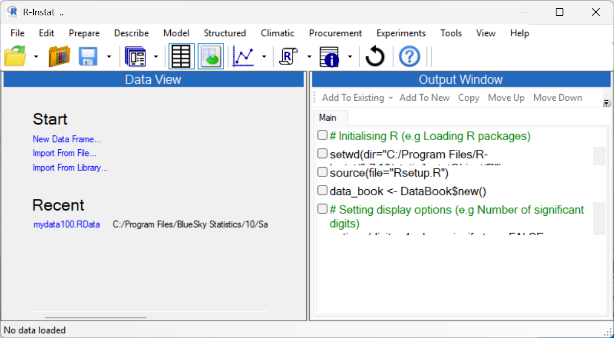
R-Instat starts up by showing its screen (Fig. 1).
Under Start, I chose “New Data Frame” and it showed me the dialog displayed in Fig. 2. I filled in some variable names, and chose their types from the drop-down menu. These were all character initially so if I had not known what a factor was, it would still have let me enter data until I figured that out.
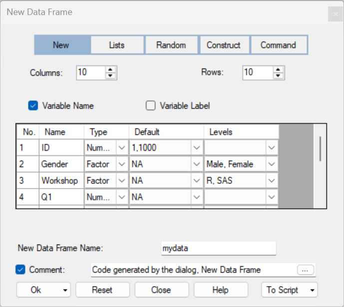
Clicking “Ok” brought up a data editor window filled with NA values for Not Available, or missing. I was then able to start entering the data. Scientific notation is accepted, but dates are saved as character variables. Logical values (TRUE, FALSE) are recognized as such and are stored appropriately. Clicking Help brought up a window that explained how a previous version of R-Instat worked. It recommended choosing “Empty,” an option replaced by “New” but it was otherwise easy to understand.
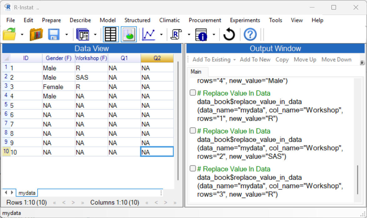
As you can see in Fig. 3, each data value I entered generated an R statement that made that happen. For users not looking to learn R, that’s an intimidating display. Most other R GUIs hide the R code unless the you ask to see it. However, the fact that it is saving R commands for every change is a valuable feature which adds to R-Instat’s reproducibility. People working in large organizations often read-access to data which they cannot correct. This enables them to read a data file and make corrections while tracking precisely what they did.
Right-clicking on any column allows you to convert a variable into a factor, ordered factor, numeric, logical, or character. These changes are recorded as function calls to a custom “convert_column_to_type” function for reproducibility. Other R GUIs do not usually record such interactive changes. Date/time conversion is unavailable on that menu, as that process is trickier. Those conversions are on the “Prepare> Column Date” menu item. You can also do from the right-click menu: rename, duplicate, reorder, set levels/labels, sort, and filter/remove filter.
The class of each variable is indicated by a character code that follows each variable name in parenthesis: (C) for character, (F) for factor, (O.F) for ordered factor, (D) for date, (L) for logical. When no code follows a variable name, it is numeric.
The name of the dataset appears on a tab at the bottom of the Data View window. This lets you easily manage multiple datasets, an ability popular among professional data analysts.
Once the dataset is saved, to add rows or columns you choose, “Prepare > Data Frame > Insert rows/columns” to add new rows or columns at any position in the data frame. New columns can be added with a specified default value, which can be a big time-saver when entering blocks of related data.
There is a quicker method that works for inserting new rows. You right-click the row numbers, and a pop-up menu will allow you to insert rows above or below. The number of rows selected is the number of rows added, like in Excel.
If you have another data set to enter, you can restart the process by choosing “File> New Data Frame” again. You can change data sets simply by clicking on its tab, and its window will pop to the front for you to see. When doing analyses or saving data, the data set displayed in the editor does not influence what appears in dialog boxes. That means that you can be looking at one dataset while analyzing another! Since each dialog allows you to choose the dataset to use, that is technically not a problem, but if you have several datasets that contain the same variable names, remember that what you see may not be what you get! That’s the opposite of BlueSky Statistics, which automatically analyzes the dataset you see. R-Instat’s ability to work with multiple datasets in a single instance of the software is not a feature found in all R GUIs. For example, jamovi and JASP can only work with a single dataset at a time.
Data is saved with a fairly standard “File> Save As> Save Dataset As” menu. By default, it will save all open datasets, filters, graphs, and models to a single file called a “data book.” That makes working with complex projects much easier to open and close.
Data Import
R-Instat supports the following file formats, most of which are automatically opened using “File> Import from File.” The ODK and NetCDF file formats have their own Import menus. R-Instat’s ability to open many formats related to climate science hints at what the software excels at. For details, see the Analysis Methods section below.
- Comma Separated Values (.csv)
- Plain text files (.txt)
- Excel (old and new xls file types)
- xBASE database files (dBase, etc.)
- SPSS (.sav)
- SAS binary files (sas7bdat and *.xpt)
- Standard R workspace files (RData, but it just opens one dataframe of its choosing)
- Open Data Kit (ODK)
- OpenRefine
- Network Common Data Form (NetCDF)
- SST Sea Surface Temperature formatted files
- IRI Data Library (API download)
- Climate Data Store (CDS) (API download)
- Shapefile
- Climsoft (Climatic database)
- .dly (ASCII files)
- .dat (ASCII files)
- Tab Separated Values (.tsv)
- Stata (.dta)
- JSON (.json)
- epiinfo (.rec)
- Minitab (.mtb)
- Systat (.syd).
- CSV with a YAML metadata header (.csvy)
- Feather R/Python interchange format (.feather)
- Pipe separated files (.psv)
- YAML (.yml)
- Weka Attribute-Relation File Format (.arff)
- Data Interchange Format (.dif)
- OpenDocument Spreadsheet (*.ods)
- Shallow XML documents (*.xml)
- Single-table HTML documents (*.html)
Data Export
The ability to export data to a wide range of file types helps when you, or other members of your research team, have to use multiple tools to complete a task. Unfortunately, this is a very weak area for most R GUIs. Deducer offers no data export at all, and R Commander and rattle can export only delimited text files (an earlier version of this listed jamovi as having very limited data export; that has now been expanded).
R-Instat has extensive export facilities. Multiple data sets can be exported:
- In a single step, as a set of files
- As a single Excel file with one data set per sheet
- As a list of data frames stored as a single RDS or RData file
- As a single HTML file with data sets end-to-end
The file formats it can export to include:
- Comma-separated file (*.csv)
- Excel files (*.xlsx
- TAB-separated data (*.tsv)
- Pipe-separated data (*.psv)
- Feather r / Python interchange format (*.feather)
- Fixed-Width format data (*.fwf)
- Serialized r objects (*.rds)
- Saved r objects (*.RData)
- JSON (*.json)
- YAML (*.yml)
- Stata (*.dta)
- SPSS (*.sav)
- XBASE database files (*.dbf)
- Weka Attribute – Relation File Format (*.arff)
- r syntax object (*.R)
- Xml (*.xml)
- HTML (*.html)
- Matlab (*.mat)
- SAS (*.sas7bdat)
- SAS XPORT (*.xpt)
Data Management
It’s often said that 80% of data analysis time is spent preparing the data. Variables need to be transformed, recoded, or created; strings and dates need to be manipulated; missing values need to be handled; datasets need to be stacked or merged, aggregated, transposed, or reshaped (e.g., from wide to long and back). A critically important aspect of data management is the ability to transform many variables simultaneously. For example, social scientists need to recode many survey items; biologists need to take the logarithms of many variables. Doing these types of tasks one variable at a time is tedious work. Some GUIs, such as JASP and RKWard, handle only a few of these functions. Others, such as BlueSky and R Commander, handle nearly all of them.
R-Instat offers one of the most comprehensive sets of data management tools of any R GUI. Its dialogs do not require any knowledge of R code. A unique feature is found in “Prepare> Check Data> Non-Numeric Values.” That detects common data entry errors in which the letter “O” is entered in place of a zero or a lowercase letter “l” in place of the number one. It offers to mark where those errors occur and optionally create a copy of the dataset with those observations deleted. Here is the list of methods it offers (some are repeated under different menus; I’ve tried to eliminate duplicates):
- Prepare> Data Frame> Rename Column
- Prepare> Data Frame> Duplicate Column
- Prepare> Data Frame> Row Numbers/Names
- Prepare> Data Frame> Sort
- Prepare> Data Frame> Filter
- Prepare> Data Frame> Column Selection
- Prepare> Data Frame> Replace Values
- Prepare> Data Frame> Convert Columns
- Prepare> Data Frame> Reorder Columns
- Prepare> Data Frame> Insert Columns/Rows
- Prepare> Data Frame> Hide/Show Columns
- Prepare> Data Frame> Column Structure
- Prepare> Data Frame> Colour by Property
- Prepare> Check Data> Visualize Data
- Prepare> Check Data> Duplicates
- Prepare> Check Data> Compare Columns
- Prepare> Check Data> Non-Numeric Values
- Prepare> Check Data> Anonymise ID Column
- Prepare> Column Calculator
- Prepare> Column Numeric> Regular Sequence
- Prepare> Column Numeric> Enter
- Prepare> Column Numeric> Row Summaries
- Prepare> Column Numeric> Transform
- Prepare> Column Numeric> Polynomials
- Prepare> Column Numeric> Random Samples
- Prepare> Column Numeric> Permute Columns
- Prepare> Column Factor> Convert to Factor
- Prepare> Column Factor> Recode to Numeric
- Prepare> Column Factor> Count in Factor
- Prepare> Column Factor> Recode Factor
- Prepare> Column Factor> Combine Factors
- Prepare> Column Factor> Dummy Variables
- Prepare> Column Factor> Levels/Labels
- Prepare> Column Factor> View Labels
- Prepare> Column Factor> Reorder Levels
- Prepare> Column Factor> Reference Level
- Prepare> Column Factor> Unused Levels
- Prepare> Column Factor> Contrasts
- Prepare> Column Factor> Factor Data Frame
- Prepare> Column Text> Find/Replace
- Prepare> Column Text> Transform
- Prepare> Column Text> Split
- Prepare> Column Text> Combine
- Prepare> Column Text> Distance
- Prepare> Column Date> Generate Dates
- Prepare> Column Date> Make Date
- Prepare> Column Date> Fill Date Gaps
- Prepare> Column Date> Use Date
- Prepare> Column Define> Convert Columns
- Prepare> Column Define> Circular
- Prepare> Data Reshape> Column Summaries
- Prepare> Data Reshape> General Summaries
- Prepare> Data Reshape> Stack (Pivot Longer)
- Prepare> Data Reshape> Unstack (Pivot Wider)
- Prepare> Data Reshape> Merge
- Prepare> Data Reshape> Append (Bind Rows)
- Prepare> Data Reshape> Subset
- Prepare> Data Reshape> Random Subset
- Prepare> Data Reshape> Transpose
- Prepare> Data Reshape> Scale/Distance
- Prepare> Keys and Links> Add Key
- Prepare> Keys and Links> View and Remove Keys
- Prepare> Keys and Links> Add Link
- Prepare> Keys and Links> View and Remove Links
- Prepare> Keys and Links> Add Comment
- Prepare> Data Object> Rename Data Frame
- Prepare> Data Object> Reorder Data Frames
- Prepare> Data Object> Copy Data Frame
- Prepare> Data Object> Delete Data Frames
- Prepare> Data Object> Hide/Snow Data Frames
- Prepare> Data Object> Metadata
- Prepare> R Objects> View
- Prepare> R Objects> Rename
- Prepare> R Objects> Reorder
- Prepare> R Objects> Delete
Menus & Dialog Boxes
The goal of pointing & clicking your way through analysis is to save time by recognizing menu settings rather than performing the more difficult task of recalling programming commands. Some GUIs, such as jamovi, make this easy by sticking to menu standards and using simpler dialog boxes; others, such as RKWard, use non-standard menus that are unique to it and hence require more learning.
R-Instat uses standard menu choices for running steps listed on its menus. Dialog boxes appear, and you select variables for their various roles. Each dialog lets you choose the dataset on a drop-down menu. Variables appear in the usual variable list box, and clicking an Add button moves the selected variables to their roles. You cannot drag variables to the various role boxes. One role box is highlighted in blue when the dialog first appears, indicating where variables will be added. You can choose a different role box by clicking on it or using the tab key to sequence through the boxes. Once a box for a single variable is filled, it automatically highlights the next variable box.
The Describe and Model menus offer a helpful labeling system of “One Variable”, “Two Variables,” “Three Variables,” and “Four Variables.” These counts include the dependent variables, so the “Three Variables” menu would allow for a model with two predictors. The default settings vary depending on the class of the variable. For example, with a numeric variable and a 2-level factor, the “Two Variables” analysis would do either a t-test or logistic regression, depending on which variable was entered first. That’s nice, but people looking on menus for a t-test or logistic regression must catch on to this approach. While the “Four Variables” items appear, they have not yet been implemented.
Once assigned, you can remove individual variables from a role assignment box. For a single variable box, press the backspace key or right-click and choose Remove to clear the box. For a multiple-variable box, select one or more variables and press the backspace key, or right-click and choose Remove for one or Clear to remove all.
The output is saved using the standard “File > Save As” menu. The only supported output format is rich text format (RTF). However, R-Instat uses that only to set the font style and color. The output tables are stored in the monospaced Courrier New font, not in true word processing tables. That is a significant failing as BlueSky, jamovi, and JASP all offer true word processing tables in the style many journals prefer. That saves you a great deal of report preparation time.
Documentation & Training
R-Instat’s documentation is listed on this web page: http://r-instat.org/ReleaseNotes.html. It includes several written and video tutorials.
Help
R GUIs provide simple task-by-task dialog boxes that generate much more complex code. So, for a particular task, you might want to get help on 1) the dialog box’s settings, 2) the custom functions it uses (if any), and 3) the R functions that the custom functions use. Nearly all R GUIs provide all three levels of help when needed. The notable exceptions are jamovi, which offers no help, and the R Commander, which lacks help on the dialog boxes themselves.
R-Instat’s help files are accessed by clicking the “Help” button on each dialog box. Unfortunately, most of these lead to empty placeholders to be filled in future versions. Those that are already filled, e.g., for renaming variables, are clear for how the dialog box works but provide no documentation on controlling the R functions it uses. The developers say all three levels of help are planned for a future release.
Graphics
The various GUIs available for R handle graphics in several ways. Some, such as RKWard, focus on R’s built-in graphics. Others, such as jamovi, use their own functions and integrate them into analysis steps. GUIs also differ greatly in how they control the style of the graphs they generate. Ideally, you could set the style once, and then all graphs would follow it. That’s how jamovi works, but then jamovi is limited to its custom graph functions, as nice as they may be.
You can generate plots in R-Instat using two different perspectives: by focusing on the number of variables involved or instead by focusing on the type of plot you wish to create. Since limiting the number of variables also limits the types of graphs that are usually considered appropriate, some may view that as the easier approach. In the “Describe> One/Two/Three Variables” menus, each provides a Graph menu choice that matches each number of variables. By choosing one variable, you’re offered bar charts, histograms, and the like. When choosing two variables, then R-Instat offers others, such as scatterplots or line plots.
You can create the same graphs by forgetting about the number of variables and instead focusing on the type of graph first. You do that under the “Describe> Specific Tables/Graphs” menu. There you will find a list of common graph types directly, such as bar, line, or scatter.
Regardless of which approach you choose to create a graph, R-Instat does most of its plots using the popular ggplot2 package. If you wish to learn R code for graphics, that’s the code you’ll see. Each graph dialog offers a “Plot Options” menu that allows you to modify the graphs in flexible and powerful ways. However, to do so requires an understanding of the Grammar of Graphics concepts, upon which R’s ggplot2 package is built. A comprehensive description of that is beyond our current scope, but it includes such complexities as a pie chart is just a bar chart with cartesian coordinates swapped out for polar ones!
One of R-Instat’s unique and useful features is its ability to save any graph, and then combine several into a single image. That makes publishing multiple graphs much easier! Currently, no other R GUI offers this feature, though the code is quite easy so I expect others will add it eventually.
Compiling a list of the plots R-Instat can do is challenging since it offers a nearly unlimited range. Here is an attempt to list the popular ones that were relatively easy to figure out how to do. Given its ability to combine plots in layers, these can be combined in many ways.
- Bar Chart of counts or pre-summarized values
- Boxplot
- Contour
- Density (continuous)
- Density (counts)
- Dumbbell
- Dot chart
- Frequency charts (factors)
- Frequency charts (numeric)
- Heatmap
- Histogram
- Line Chart
- Line Chart, stair-step plot
- Line Chart, variable order
- Maps: World Map
- Mosaic
- Parallel Coordinate Plot
- Pie Chart
- Plot of Means
- Polar Coordinate Plots
- P-P Plots
- Q-Q Plots
- Scatterplot
- Scatterplot matrix
- Strip Chart
- TreeMap
- Violin Plot
- Word Cloud
- Visualize dataset by variable type & missing values
- Stacked rating data
- Barchart of Likert variable percents
- Climatic> PISCA> General Graph
- Climatic> PICSA> Rainfall Graph
- Climatic> PICSA> Temperature Graph
- Climatic> PICSA> Cumulative/Exceedance Graph
- Climatic> PICSA> Crops
- Structured> Circular> Circular Plots
- Structured> Circular> Wind Rose
- Structured> Circular> Wind/Polution Rose
- Structured> Circular> Other Rose Plots
Let’s take a look at how R-Instat does scatterplots. Using the dialog box “Describe> Graphs> Scatter Plot” I chose only the “X” variable and the “Single Variable” (an odd name for the Y variable on this dialog), row facet factor, column facet factor, the type of smoothing fit, and checked a box to plot standard errors. The facets created six “small multiples” of the plot, making comparisons easy. Other R GUIs include the ability to do “large multiples” of plots by any number of other factor variables, e.g. BlueSky’s “Datasets> Group-by” dialog. R-Instat lacks that useful feature. Here is the code that R-Instat wrote, followed by the plot (Fig. 4) it made:
require(ggplot2);
require(ggthemes);
require(stringr);

## [Scatterplot (Points)]
ggplot(data=mydata100, aes(x=pretest,y=posttest)) +
	geom_point() +
	geom_smooth( method ="lm", alpha=1, se=TRUE,) +
	labs(x="pretest",y="posttest",
title= "Scatterplot for X axis: pretest ,Y axis: posttest ") +
	xlab("pretest") +
	ylab("posttest") +
	theme_gray() +
	theme(text=element_text(family="serif",
	face="plain",
	color="#000000",size=12,
	hjust=0.5,vjust=0.5))
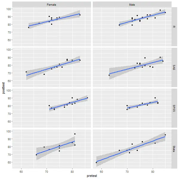
There is some naming confusion, in which the menu called this a scatter plot, but the title in the output labeled it a point plot. That could make it hard to recall which menu choice was responsible for making the plot.
R-Instat exports graphs using the “File> Export> Export Graph as Image.” It offers the following file formats, which include almost any format you could need:
- JPEG
- PNG
- BitMap
- EPS
- Postscript
- SVG
- WMF
Modeling
The way statistical models (which R stores in “model objects”) are created and used is an area on which R GUIs differ the most. The simplest and least flexible approach is taken by jamovi and RKWard. They try to do everything you might need in a single dialog box. They either don’t save models, or they do nothing with them. To an R programmer, that sounds extreme since R does a lot with model objects. However, neither SAS nor SPSS could save models for the first 35 years of existence, so each approach has its merits. For simple models like linear regression, standard compute statements can make predictions. Entering them manually is not much effort, and it saves you from learning what a model object is. However, some of the most powerful model types, such as neural networks, random forests, and gradient-boosting machines, are impossible to enter by hand.
R-Instat’s “Model> Fit Model” menu offers menus named from One Variable to Four Variables. Those counts include the dependent variable, so a three-variable model would allow for two independent variables. By default, additive models are fit, but a Model Operator menu allows you to choose options such as the “:” to generate interactions. However, it does not explain what those operators do, so you must learn what they mean in R if you wish to do anything beyond a simple additive model. A Model Preview window shows you the model it is writing, and it also allows you to type your model in, assuming you know R model syntax.
Each dialog also allows you to choose the distributions from: Normal, Poisson, Gamma, Inverse Gaussian, Quasi, and Quasi-Poisson. Additionally, each allows the choice of link functions: identity, log, logit, cloglog, sqrt, 1/mu^2, Cauchit, Probit, and Inverse. Such complex options are usually divided into separate focused dialogs in the other R GUIs.You make your selections and click the Return button to exit to the main dialog.
An alternative approach to model building uses the General menu. It simply offers an Explanatory Model field rather than prompts for first and second predictor variables. The model-building tools are basic, with the Add button moving a variable and other buttons adding operators such as “+” or “/”. Other software, such as jamovi and BlueSky offer ways to enter a set of variables, each separated by any operator you choose. They also let you add all possible 2-, 3-, or N-way interactions to models, which speeds up your work with complex models.
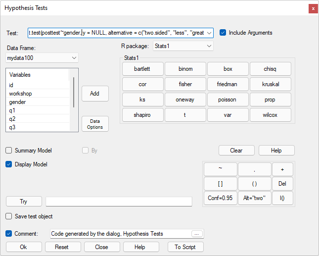
The third approach to model building is the Hypothesis Test Keyboard, shown in Fig. 5. I’m using it to perform a t-test. This is the dialog used for the most common statistical tests. I opened it using “Model> Fit Model> Hypothesis Test Keyboards.” The “Stats1” R package was the default, and I checked the “Include Arguments” box. When I clicked on the “t” button to perform a t-test, the full R syntax for the “t.test.” function appeared in the Test box. I applied my knowledge of R and replaced the “x=” argument that it had offered with “posttest ~ gender” to compare males and females on a posttest score. I used the Add and “~” buttons, but it would have been faster to simply type the formula without that assistance. For such widely-used tests, this dialog offers nothing like the easy-to-use dialogs of all of the other R GUIs reviewed in this series.
A fourth approach involves the use of a Model Keyboard, shown in Fig. 6. Here, I’m using it to perform a robust linear regression. Knowing that the MASS package offers it, I chose that from the Package menu. I then clicked the Include Arguments checkbox, then I clicked the rlm button. The full syntax is filled in as shown. I typed in “posttest ~ pretest” as my model and clicked OK to run it. However, the default settings of the other arguments generated an error, so I deleted all arguments except for the formula. I did it this way to demonstrate that while R-Instat provides valuable assistance, you must still know the basics of the R language to make the most of it.
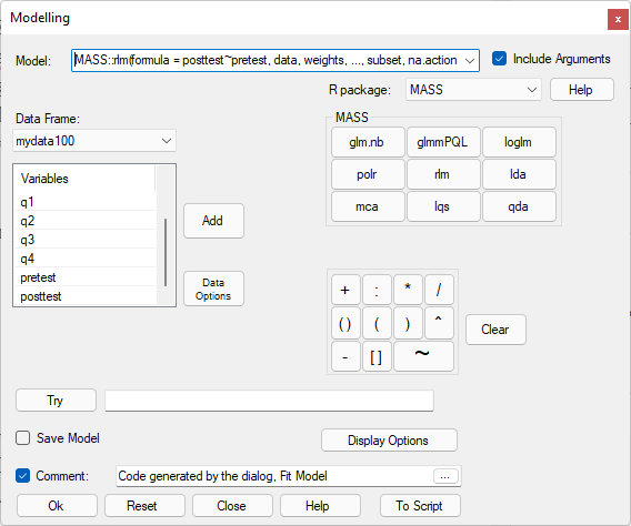
the MASS package’s rlm function.
The models R-Instat creates are stored in a unique “data book” structure. This approach makes it easy to use models within R-Instat and easy to save them along with the dataset(s) in its databook format. There are also ways to export models from the data books into standard R objects for use outside R-Instat.
The menu item “Model> Compare Models> One Variable” lets you compare two models, but only those that compare a single variable to a distribution. The developers plan to expand this to all model types that R-Instat can create (where mathematically possible).
The “Model> Use Model” menu lets you use saved models to do things like making predictions on new datasets. This is often the main point of creating a model, so I find it surprising that only a few R GUIs provide this capability! This menu also includes the very useful ability to glance, tidy, or augment a model. This is the broom package’s terminology for summarizing a model at the model, parameter, or observation level. The addition of a “by” factor would be helpful for those.
To summarize, R-Instat trades off ease of use for power. While most other GUIs prevent you from knowing any R code, they must provide a dialog for every situation. R-Instat’s approach is very general, allowing you to run a vast array of models from just a handful of dialogs. However, you must know the R packages and how their functions work even when performing basic statistical tests.
Analysis Methods
All of the R GUIs offer a set of statistical analysis methods. Some also offer machine learning methods. As you can see in the table below, R-Instat offers an extensive set of statistical analysis methods but no machine learning. As with R-Instat’s graphics, its analytic ability can access the same analysis in multiple ways. Here is a comprehensive list of its analysis methods in which I list each technique once. Remember that many of these methods simply generate R code that you will need to edit to control options.
- Describe> One Variable> Summary stats
- Describe> One Variable> Frequencies
- Describe> One Variable> Rating data (frequencies & percents on many vars in one table)
- Describe> Two Variables> Frequencies does crosstabs but no tests
- Describe> Three Variables> Frequencies does crosstabs but no CMH test
- Describe> Three Variables> Pivot Table creates interactive tables
- Describe> Multivariate> Correlations – Pearson
- Describe> Multivariate> Correlations – Nonparametric Kendall, Spearman
- Describe> Multivariate> Principle Components
- Describe> Multivariate> Canonical Correlations
- Hypothesis Tests> Stats1> bartlet
- Hypothesis Tests> Stats1> binom
- Hypothesis Tests> Stats1> box
- Hypothesis Tests> Stats1> chisq
- Hypothesis Tests> Stats1> cor
- Hypothesis Tests> Stats1> fisher
- Hypothesis Tests> Stats1> friedman
- Hypothesis Tests> Stats1> kruskal
- Hypothesis Tests> Stats1> ks
- Hypothesis Tests> Stats1> oneway
- Hypothesis Tests> Stats1> poisson
- Hypothesis Tests> Stats1> prop
- Hypothesis Tests> Stats1> shapiro
- Hypothesis Tests> Stats1> t
- Hypothesis Tests> Stats1> var
- Hypothesis Tests> Stats1> wilcox
- Hypothesis Tests> Stats2> ansari
- Hypothesis Tests> Stats2> fligner
- Hypothesis Tests> Stats2> mantelhaen
- Hypothesis Tests> Stats2> mauchly
- Hypothesis Tests> Stats2> mcnemar
- Hypothesis Tests> Stats2> mood
- Hypothesis Tests> Stats2> pairwise.Prop
- Hypothesis Tests> Stats2> pairwise.wilcox
- Hypothesis Tests> Stats2> pairwise.t
- Hypothesis Tests> Stats2> power.anova
- Hypothesis Tests> Stats2> power.prop
- Hypothesis Tests> Stats2> power.t
- Hypothesis Tests> Stats2> prop.trend
- Hypothesis Tests> Stats2> PP
- Hypothesis Tests> Stats2> quade
- Hypothesis Tests> Stats2> Clear
- Hypothesis Tests> Agricolae> BIB
- Hypothesis Tests> Agricolae> duncan
- Hypothesis Tests> Agricolae> durbin
- Hypothesis Tests> Agricolae> friedman
- Hypothesis Tests> Agricolae> kruskal
- Hypothesis Tests> Agricolae> LSD
- Hypothesis Tests> Agricolae> median
- Hypothesis Tests> Agricolae> nonadditivity
- Hypothesis Tests> Agricolae> PBIB
- Hypothesis Tests> Agricolae> REGW
- Hypothesis Tests> Agricolae> scheffe
- Hypothesis Tests> Agricolae> SNK
- Hypothesis Tests> Agricolae> waerden
- Hypothesis Tests> Agricolae> waller
- Hypothesis Tests> Verification> binary
- Hypothesis Tests> Verification> cat
- Hypothesis Tests> Verification> cont
- Hypothesis Tests> Coin> oneway
- Hypothesis Tests> Coin> wilcox
- Hypothesis Tests> Coin> kruskal
- Hypothesis Tests> Coin> normal
- Hypothesis Tests> Coin> median
- Hypothesis Tests> Coin> savage
- Hypothesis Tests> Coin> sign
- Hypothesis Tests> Coin> wilcoxsign
- Hypothesis Tests> Coin> friedman
- Hypothesis Tests> Coin> quade
- Hypothesis Tests> Coin> taha
- Hypothesis Tests> Coin> mood
- Hypothesis Tests> Coin> flinger
- Hypothesis Tests> Coin> klotz
- Hypothesis Tests> Coin> ansari
- Hypothesis Tests> Coin> conover
- Hypothesis Tests> Coin> spearman
- Hypothesis Tests> Coin> quadrant
- Hypothesis Tests> Coin> fisyat
- Hypothesis Tests> Coin> koziol
- Hypothesis Tests> Coin> chisq
- Hypothesis Tests> Coin> cmh
- Hypothesis Tests> Coin> lbl
- Hypothesis Tests> Trend> bartels
- Hypothesis Tests> Trend> br
- Hypothesis Tests> Trend> bu
- Hypothesis Tests> Trend> cs
- Hypothesis Tests> Trend> csmk
- Hypothesis Tests> Trend> lanzante
- Hypothesis Tests> Trend> mk
- Hypothesis Tests> Trend> mmk
- Hypothesis Tests> Trend> pcor
- Hypothesis Tests> Trend> pmk
- Hypothesis Tests> Trend> pettitt
- Hypothesis Tests> Trend> rrod
- Hypothesis Tests> Trend> ssens
- Hypothesis Tests> Trend> sens
- Hypothesis Tests> Trend> smk
- Hypothesis Tests> Trend> snh
- Hypothesis Tests> Trend> wm
- Hypothesis Tests> Trend> ww
- Model> Probability Distributions> Normal
- Model> Probability Distributions> Exponential
- Model> Probability Distributions> Geometric
- Model> Probability Distributions> Weibull
- Model> Probability Distributions> Uniform
- Model> Probability Distributions> Bernouli
- Model> Probability Distributions> Binomial
- Model> Probability Distributions> Poisson
- Model> Probability Distributions> Beta
- Model> Probability Distributions> Negative Binomial
- Model> Probability Distributions> Student’s t
- Model> Probability Distributions> von Mises
- Model> Probability Distributions> Cauchy
- Model> Probability Distributions> Chi Square
- Model> Probability Distributions> F
- Model> Probability Distributions> Lognormal
- Model> Probability Distributions> Gamma
- Model> Probability Distributions> Extreme Value
- Model> Probability Distributions> Generalized Pareto
- Model> Probability Distributions> Gumbel
- Modeling> stats> aov
- Modeling> stats> ar
- Modeling> stats> arima
- Modeling> stats> glm
- Modeling> stats> lm
- Modeling> stats> loess
- Modeling> stats> loglin
- Modeling> stats> lowess
- Modeling> stats> spline
- Modeling> stats> nls
- Modeling> stats> ppr
- Modeling> stats> princomp
- Modeling> extRemes> fevd
- Modeling> extRemes> levd
- Modeling> lme4> glmer
- Modeling> lme4> lemr
- Modeling> lme4> nlmer
- Modeling> MASS> glm.nb
- Modeling> MASS> glmmPQL
- Modeling> MASS> loglm
- Modeling> MASS> polr
- Modeling> MASS> rlm
- Modeling> MASS> lda
- Modeling> MASS> mca
- Modeling> MASS> lqs
- Modeling> MASS> qda
- Structured> Circular> Define
- Structured> Circular> Calculator
- Structured> Circular> Summaries
- Structured> Low Flow> Define
- Structured> Survival> Define
- Structured> Time Series> Define
- Structured> Time Series> Describe> One Variable
- Structured> Time Series> Describe> General
- Structured> Time Series> Model> One Variable
- Structured> Time Series> Model> General
- Structured> Climatic
- Structured> Procurement
- Structured> Options by Context
- Climatic> Check Data> Inventory
- Climatic> Check Data> Display Daily
- Climatic> Check Data> Fill Missing Values
- Climatic> Check Data> QC Temperatures
- Climatic> Check Data> QC Rainfall
- Climatic> Check Data> Homogenization
- Climatic> Check Data> Check Station Locations
- Climatic> Prepare> Climatic Summaries
- Climatic> Check Data> Start of Rains
- Climatic> Check Data> End of Rains
- Climatic> Check Data> Length of Season
- Climatic> Check Data> Spells
- Climatic> Check Data> Extremes
- Climatic> Check Data> Climdex
- Climatic> Check Data> SPI/SPEI
- Climatic> Check Data> Evapotranspiration
- Climatic> Describe> Rainfall
- Climatic> Describe> Temperature
- Climatic> Describe> Wind Speed/Direction
- Climatic> Describe> Sunshine/Radiation
- Climatic> Describe> General
- Climatic> NCMP> Indices
- Climatic> NCMP> Variogram
- Climatic> NCMP> Region Average
- Climatic> NCMP> Trend Graphs
- Climatic> NCMP> Count Records
- Climatic> NCMP> Summary
- Climatic> Plot Region
- Climatic> Compare> Calculation
- Climatic> Compare> Summary
- Climatic> Compare> Correlations
- Climatic> Compare> Scatterplot
- Climatic> Compare> Time Series Plot
- Climatic> Compare> Seasonal Plot
- Climatic> Compare> Conditional Quantiles
- Climatic> Compare> Taylor Diagram
- Climatic> Mapping> Maps
- Climatic> Mapping> Check Station Locations
- Climatic> Model> Extremes
- Climatic> Model> Markov Modelling
- Climatic> Seasonal Forecast Support> Cumulative/Exceedance Graph
- Procurement> Prepare> Define Contract Value Categories
- Procurement> Prepare> Recode Numeric into Quantiles
- Procurement> Prepare> Use Award Date (or other)
- Procurement> Prepare> Summarise Red Flags by Country (or other)
- Procurement> Prepare> Summarise Red Flags by Country and Year (or other)
- Procurement> Corruption Risk Index (CRI)> Define Corruption Risk Index (CRI)
Generated R Code
One of the aspects that most differentiates the various GUIs for R is the code they generate. If you decide to save code, what type is best for you? The base R code, as provided by the R Commander that can teach you “classic” R? The concise functions that mimic the simplicity of one-step dialogs, as jamovi provides? The completely transparent (and complex) code provided by RKWard, which might be the best for budding R power users?
R-Instat writes a blend of custom functions and functions from the popular tidyverse package. As mentioned previously, it uses ggplot2 for graphics.
Here’s an example of code R-Instat wrote to do a group-by aggregation:
data_book$calculate_summary(data_name="mydata1001", columns_to_summarise=c("pretest","posttest"), factors=c("workshop","gender"), j=1, summaries=c("summary_mean"), silent=TRUE)
Here is an example of code R-Instat wrote to convert my “wide” style dataset to a “long” one. The wide one had measurements at four times, stored in variables named q1 through q4. I wanted those stacked into a single variable named “Score” and the variable names written into a factor called “Time.” The code R-Instat generated is below. It used the tidyr package’s pivot_longer function, just as I would have. However, that is only one of four function calls used; the rest are for internal use of R-Instat. Beginners looking to learn R must sift through these to determine which performed the actual task. When I tried to unstack this new dataset back into its original form, the dialog would not accept the variable Time, since it was not a factor. Given that R-Instat had just created it, it should have made it one to ease a “round trip” conversion, which is a fairly common task to perform (variable selections along the way don’t necessarily result in a complete duplicate of the original dataset). The developers plan to make that a factor in a future release.
# Code generated by the dialog, Stack (Pivot Longer)

mydata1001 <- data_book$get_data_frame(data_name="mydata1001")

mydata1001_stacked <- tidyr::pivot_longer(data=mydata1001, cols=c("q1","q2","q3","q4"), names_to="Time",  values_to="Score")

data_book$import_data(data_tables=list(mydata1001_stacked=mydata1001_stacked))

rm(list=c("mydata1001_stacked", "mydata1001"))
Below is an example of R-Instat’s code and output for a simple linear regression. The computations use the same functions as any R programmer would choose (i.e., those included with R itself). As before, you need to know which those are to separate them from R-Instat’s internal function calls.
# Code generated by the dialog, Two Variable Fit Model
mydata1001_stacked1 <- data_book$get_data_frame(data_name="mydata1001_stacked1")

attach(what=mydata1001_stacked1)

two_var <- lm(data=mydata1001_stacked1, formula=posttest ~ pretest, na.action=na.exclude)

data_book$add_model(model_name="two_var", model=two_var, data_name="mydata1001_stacked1")
data_book$get_models(data_name="mydata1001_stacked1", model_name="two_var")


Call:
lm(formula = posttest ~ pretest, data = mydata1001_stacked1,
    na.action = na.exclude)

Coefficients:
(Intercept)      pretest
     18.665        0.846


stats::anova(object=data_book$get_models(data_name="mydata1001_stacked1", model_name="two_var"))

Analysis of Variance Table

Response: posttest
           Df Sum Sq Mean Sq F value Pr(>F)
pretest     1   7943    7943     342 <2e-16
Residuals 398   9256      23

summary(object=data_book$get_models(data_name="mydata1001_stacked1", model_name="two_var"))


Call:
lm(formula = posttest ~ pretest, data = mydata1001_stacked1,
    na.action = na.exclude)

Residuals:
   Min     1Q Median     3Q    Max
-9.313 -4.025 -0.435  3.780 11.297

Coefficients:
            Estimate Std. Error t value Pr(>|t|)
(Intercept)  18.6647     3.4389    5.43    1e-07
pretest       0.8456     0.0458   18.48   <2e-16

Residual standard error: 4.82 on 398 degrees of freedom
Multiple R-squared:  0.462,	Adjusted R-squared:  0.46
F-statistic:  342 on 1 and 398 DF,  p-value: <2e-16


detach(name=mydata1001_stacked1, unload=TRUE)

rm(list=c("two_var", "mydata1001_stacked1"))
Support for Programmers
Some R GUIs reviewed in this series of articles include extensive support for programmers. For example, RKWard offers much of the power of Integrated Development Environments (IDEs) such as RStudio or Eclipse StatET. Others, such as jamovi or the R Commander, offer little more than a simple text editor.
R-Instat has a script window that lets you do basic programming. A “Run” button lets you step through a program one line at a time or click “Run All.” There are no additional features such as syntax color-coding, code-completion suggestions, or search or replace functions. While most GUI users are not likely to write extensive programs, a few more basics would be helpful.
The R-Instat developers view the current script window as primarily for “tweaking” the R command generated by each dialog rather than for writing code from scratch. Dialogs have a “To Script” button populating the script window with working code, ready to be examined and possibly edited before execution. They also have a short guide called “Reading, tweaking and using R commands” to help learn these steps.
Reproducibility & Sharing
One of the biggest challenges that GUI users face is being able to reproduce their work. Reproducibility is useful for re-running everything on the same dataset if you find a data entry error. It’s also useful for applying your work to new datasets so long as they use the same variable names (or if the software can handle name changes). Some scientific journals ask researchers to submit their files (usually code and data) and written reports so that others can check their work.
As important a topic as it is, reproducibility is a problem for GUI users, a problem that has only recently been solved by some software developers. Most GUIs (e.g. the R Commander, Rattle) save only code, but since the GUI user didn’t write the code, they also can’t read it or change it! Others, such as BlueSky, jamovi, JASP, and RKWard, save the dialog box entries, allowing GUI users reproducibility in their preferred form.
R-Instat’s Output window contains all the code created by the GUI. As mentioned above, it goes above and beyond what most GUIs save by including every interactive change a user might make to the data via manual data entry or right-click menus to convert, say, numeric variables to factors. However, it remembers only the details of the last ten dialogs you run.
If you wish to share your work with a colleague who also uses R-Instat, you would save the contents of your log file (viewable under “View> Log Window”) and send them that script and your dataset. They would then edit the path in the R code to point to the location of the data file on their computer.
To share your work with a colleague who uses RStudio, or a similar IDE, you would send them your log and data files. Your colleague would install R-Instat to get its set of custom functions (these are not in an R package on CRAN, though that is the long-term plan). The script saved from the log window includes a pointer to the location of those functions on the person’s hard drive.
Package Management
A topic related to reproducibility is package management. One of the major advantages to the R language is that it’s very easy to extend its capabilities through add-on packages. However, updates in these packages may break a previously functioning analysis. Years from now, you may need to run a variation of an analysis, which would require you to find the version of R you used, plus the packages you used at the time. As a GUI user, you’d also need to find the version of the GUI that was compatible with that version of R.
Some GUIs, such as the R Commander and Deducer, depend on you to find and install R. For them, the long-term stability problem is yours to solve. Others, such as jamovi, distribute their version of R and all R packages but not their add-on modules. This requires a bigger installation file, but it makes dealing with long-term stability simpler. Of course, this depends on all major versions being around for the long term. Still, for open-source software, multiple archives are usually available to store software, even if the original project is defunct.
R-Instats approach to package management is one of the most comprehensive of the R GUIs reviewed here. It provides everything you need in a single download. This includes the R-Instat interface, R itself, and all the necessary R packages. If you have a problem reproducing an R-Instat analysis in the future, you only need to download the version used when you created it.
Output & Report Writing
Ideally, output should be clearly labeled, well organized, and of publication quality. It might also delve into word processing through the use of Markdown or LaTeX. You can now get publication-quality output from BlueSky, Deducer, jamovi, and JASP. You can also get LaTeX output from BlueSky. jamovi, JASP, and RKWard.
Unfortunately, R-Instat’s tabular output is in R’s standard text tables. These must be displayed using a monospaced font to keep the columns lined up. While R packages such as gt, texreg, and xtable exist to convert these tables to publication quality, that step would require writing R code. The R-Instat developers say they plan to add publication-quality output in a future version.
Group-By Analyses
Repeating an analysis on different groups of observations is a core task in data science. Software needs to provide the ability to select a subset of one group to analyze, then another subset to compare it to. All the R GUIs reviewed in this series can do this task. R-Instat does single-group selections by offering to filter rows using the “Data Options” button in every dialog. It generates a subset that you can analyze in the same way as the entire dataset.
Software also needs the ability to automate such selections so that you might generate dozens of analyses or graphs, one group at a time. This feature has been available in commercial GUIs for decades (e.g., SPSS split-file, SAS BY). R-Instat does not offer such a feature.
Output Management
Early in the development of statistical software, developers tried to guess what output would be important to save to a new dataset (e.g., predicted values, factor scores), and the ability to save such output was built into the analysis procedures themselves. However, researchers were far more creative than the developers anticipated. To better meet their needs, output management systems were created and tacked on to existing tools (e.g., SAS’ Output Delivery System, SPSS’ Output Management System). One of R’s greatest strengths is that every bit of output can be readily used as input. However, with the simplification that GUIs provide, that presents a challenge.
Output data can be observation-level, such as predicted values for each observation or case. When group-by analyses are run, the output data can also be observation-level, but now the (e.g.) predicted values would be created by individual models for each group rather than one model based on the entire original data set (perhaps with group included as a set of indicator variables).
Group-by analyses can also create model-level data sets, such as one R-squared value for each group’s model. They can also create parameter-level data sets, such as the p-value for each regression parameter for each group’s model. (Saving and using single models is covered under “Modeling” above.)
For example, in our organization, we have 250 departments and want to see if any have a gender bias on salary. We write all 250 regression models to a data set and then search to find those whose gender parameter is significant (hoping to find none, of course!)
R-Instat does all three levels of output management. To use this function, choose “Model> Use Model> Glance/Tidy/Augment.” While the code to repeat this for the levels of one or more grouping variables is fairly easy to implement, the dialog doesn’t currently offer that feature.
Developer Issues
The R-Instat team welcomes people who are willing to contribute to the project. You can submit bug reports or even copy the entire set of source code at the project’s GitHub site: https://github.com/africanmathsinitiative/R-Instat/. Information and guides for developers and contributors are available on the GitHub Wiki: https://github.com/africanmathsinitiative/R-Instat/wiki
Conclusion
R-Instat offers one of the most extensive collections of data wrangling, graphics, and statistical analysis methods of any R GUI. Its data wrangling dialogs are simple to use and require no knowledge of R code. At a basic level, its graphics and modeling dialogs are also easy to use. However, its dependence on R code for basic statistical methods such as chi-squared or t-tests makes it far more difficult to use than other R GUIs. To use its full modeling capabilities, you need to know what R’s packages (e.g., MASS) are and what each one’s functions (e.g., rlm) do. For an R programmer, recognizing a known package::function combination is much easier than recalling it without assistance. Such a user would find R-Instat’s GUI extremely helpful. R-Instat’s ability to add ggplot2 layers allows you to create a graph of nearly unlimited flexibility. But you need to learn the difference between functions like geom_line and geom_smooth to take full advantage of it.
R-Instat’s offering in climate analysis is unique among R GUIs, and a quick search on Google Scholar shows that it is being widely used with such data. R-Instat focuses on frequentist statistics rather than Bayesian, and it does not yet offer any machine learning or artificial intelligence methods. R-Instat’s developers are currently working to include some machine learning methods using the caret package, particularly for teaching data science.
R-Instat’s output is in standard R text tables, rather than the journal-style word processing tables that are such a time-saver in other R GUIs.
If you have an R programming background or want to learn R code, R-Instat may be just what you need to get started.
The R-Instat team wrote a detailed response to this review, which is online here. For a summary of all my R GUI software reviews, see the article, R Graphical User Interface Comparison.
Acknowledgments
Thanks to the R-Instat team, who have done a lot of hard work and for making it free and open source. Thanks to David Stern, Roger Stern, and Danny Parsons for clarifying many aspects of R-Instat. Also, to Rachel Ladd, Ruben Ortiz, Christina Peterson, and Josh Price for their editorial suggestions.