by Robert A. Muenchen, updated July 9, 2026
Introduction
RKWard is a free and open-source Graphical User Interface for the R software, one that supports beginners looking to point-and-click their way through analyses, as well as advanced programmers. You can think of it as a blend of the menus and dialog boxes that R Commander offers combined with the programming support that RStudio provides. RKWard is available on Windows, Mac, and Linux. However, the Mac version has problems, as described by the RKWard Mac webpage: “The 0.8.0 version of RKWard on Mac is known to crash during startup, occasionally, for reasons still under investigation. Please just try again. Once successfully started, RKWard should work, reliably.”
This review is one of a series which aims to help non-programmers choose the Graphical User Interface (GUI) that is best for them. However, I do include a cursory overview of how RKWard helps you work with code. In most sections, I’ll begin with a brief description of the topic’s functionality and how GUIs differ in implementing it. Then I’ll cover how RKWard does it.
I have joined the BlueSky Statistics development team and have written the BlueSky User Guide (online here), but you can trust this series of reviews, as I describe here. All my comments below are easily verifiable. There is no perfect user interface for everyone; each GUI for R has features that appeal to different people.
Terminology
There are various definitions of user interface types, so here’s how I’ll be using the following terms. Reviewing R GUIs keeps me quite busy, so I don’t have time also to review all the IDEs, though my favorite is RStudio.
GUI = Graphical User Interface, specifically using menus and dialog boxes to avoid having to type programming code. I do not include any assistance for programming in this definition. So GUI users are people who prefer using a GUI to perform their analyses. They often don’t have the time required to become good programmers.
IDE = Integrated Development Environment which helps programmers write code. I do not include point-and-click style menus and dialog boxes when using this term. IDE users are people who prefer to write R code to perform their analyses.
Installation
The various user interfaces available for R differ quite a lot in how they’re installed. Some, such as jamovi or BlueSky Statistics, install in a single step. Others install in multiple steps, such as R Commander and Deducer. Advanced computer users often don’t appreciate how lost beginners can become while attempting even a single-step installation. I work at the University of Tennessee, and our HelpDesk is flooded with such calls at the beginning of each semester!
Installing RKWard on Windows is done in a single step since its installation file contains both R and RKWard. Linux binaries do not contain a matching copy of R, but the package manager will obtain R (unless already installed). On Mac, the user is responsible for installing R manually. Regardless of their operating system, RKWard users never need to learn how to start R, then execute the install.packages function, and then load a library.
The RKWard installer obtains the appropriate version of R, simplifying the installation and ensuring complete compatibility. However, if you already had a copy of R installed, depending on its version, you could end up with a second copy.
RKWard minimizes the size of its download by waiting to install some R packages until you actually try to use them for the first time. Then it prompts you, offering default settings that will get the package you need.
Plug-ins
When choosing a GUI, one of the most fundamental questions is: what can it do for you? What the initial software installation of each GUI gets you is covered in the Graphics, Analysis, and Modeling section of this series of articles. Regardless of what comes built-in, it’s good to know how active the development community is. They contribute “plug-ins” that add new menus and dialog boxes to the GUI. This level of activity ranges from very low (RKWard, BlueSky, Deducer) through moderate (jamovi) to very active (R Commander).
Currently, all plug-ins are included with the initial installation. You can see them using the menu selection Settings> Configure Packages> Manage RKWard Plugins. There are only brief descriptions of what they do, but once installed, you can access the help files with a single click.
RKWard add-on modules are part of standard R packages and are distributed on CRAN. Their package descriptions include a field labeled “enhances: rkward”. You can sort packages by that field in RKWard’s package installation dialog, which displays them with the RKWard icon.
Startup
Some user interfaces for R, such as jamovi and BlueSky Statistics, start by double-clicking on a single icon, which is great for people who prefer not to write code. Others, such as R commander, have you start R, then load a package from your library, then call a function. That’s not good for GUI users, but for people looking to learn the R language, it helps them on their way.
RKWard is started directly as a stand-alone application, not from within R. The next time you start it up, it offers to load your last open workspace & it knows its location.
Data Editor
A data editor is a fundamental feature in data analysis software. It puts you in touch with your data and lets you get a feel for it, if only in a rough way. A data editor is such a simple concept that you might think there would be hardly any differences in how they work in different GUIs. While there are technical differences, to a beginner, what matters the most are the differences in simplicity. Some GUIs, including jamovi and Bluesky, let you create only what R calls a data frame. They use more common terminology and call it a dataset: you create one, you save one, later you open one, then you use one. Others, such as the R Commander, trade this simplicity for the full R language perspective: a data set is stored in a workspace. So the process goes: you create a data set, you save a workspace, you open a workspace, and then choose a data set from within it.
RKWard’s spreadsheet-style data editor is very easy to use. It puts its metadata – variable name, label, type, format, and levels – at the top of each variable (Figure 2). This makes it seem quite natural that you start at the top of the spreadsheet and work your way down until you’re entering the data values. Under “Type” you can double-click to reveal a dropdown menu that shows 1:Numeric, 2:Factor, 3:String, and 4:Logical. You can either click on one of those choices or type its number to make the selection.
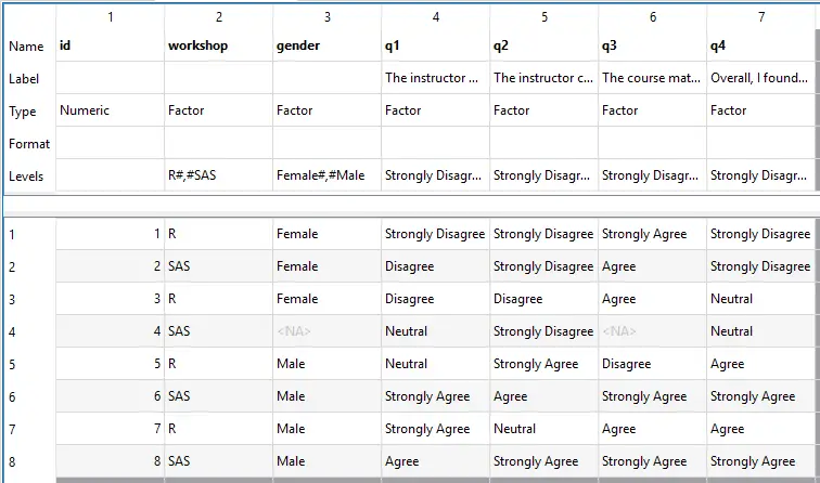
Double-clicking “Levels” opens a dialog that offers values of a factor, such as 1 or 2, and prompts you to enter each label, such as Male or Female. When finished, you can then continue with data entry, typing numbers, and having RKWard convert their numbers to the labels. That makes data entry quick and accurate.
The tab key takes you to the next cell. It also adds a new variable when you reach the end of the defined variables. That’s handy if it’s what you want to do, but it’s also easy to create a new variable by accident. If that happens, right-click on the variable name and choose “delete.”
The Home and End keys take you to the beginning or end of an observation. So to begin entering a new observation, you press Home, then cursor down (or vice versa). I would prefer that the Enter key be used in place of that two-key sequence, but Excel users will probably like it as is.
To save your dataset, choose Workspace> Save Workspace. Recall that to start creating a dataset, you use File> New> Dataset. Since there’s no matching File> Save> Dataset, the beginner is left to make the mental leap that a workspace is the thing that needs saving!
When opening an existing data set, most programs will show you the data in spreadsheet form, but RKWard doesn’t. The file opens into a new tabbed window, but that window does not pop to the front, making you wonder if you succeeded in opening the file or not. Another way you’ll know it opened is that its name appears in the Workspace window in the upper left of the main control window.
Data Import / Export
RKward offers a limited selection of data import & export formats:
- Delimited Values (.csv, .tsv)
- Plain text files (.txt)
- Excel (old and new xls file types)
- SPSS (.sav)
- Standard R workspace files (.RData)
Data Management
It’s often said that 80% of data analysis time is spent preparing the data. Variables need to be transformed, recoded, or created; missing values need to be handled; datasets need to be stacked or merged, aggregated, transposed, or reshaped (e.g. from wide to long and back). An essential aspect of data management is the ability to transform many variables simultaneously. For example, social scientists need to recode many survey items; biologists need to take the logarithms of many variables. Doing such tasks one variable at a time is tedious. Some GUIs, such as R Commander and BlueSky Statistics, handle nearly all of these challenges. Others, such as JASP, offer just a handful of data management functions.
RKWard’s collection data mangement features is one of the most powerful of any of the R GUIs. Its Data menu offers the following choices:
- ANOVA > Prepare within-subject data
- Class and Structure > Batch Column Conversion
- Class and Structure > Coerce Data Structure
- Class and Structure > Coerce Vector Type
- Class and Structure > Manipulate Lists > Create or Append List
- Class and Structure > Manipulate Lists > Extract List Elements
- Combine Data Tables (dplyr) > Combine by Binding
- Combine Data Tables (dplyr) > Filtering Joins
- Combine Data Tables (dplyr) > Mutating Joins
- Combine Data Tables (dplyr) > Set Operations
- Data Cleaning (janitor) > Clean Data
- Data Cleaning (janitor) > Frequency Tables
- Data Cleaning (janitor) > Inspect Cases
- Data Cleaning (janitor) > Manage Duplicates
- Data Wrangling > Batch Recode
- Data Wrangling > Batch Transform
- Data Wrangling > Create Composite Score
- Data Wrangling > Create Dummy Variables (fastDummies)
- Date and Time (lubridate) > Apply Stamp Function
- Date and Time (lubridate) > Calculations > Advanced Extractions
- Date and Time (lubridate) > Calculations > Align Dates
- Date and Time (lubridate) > Calculations > Check Overlaps
- Date and Time (lubridate) > Calculations > Decimal Conversion
- Date and Time (lubridate) > Calculations > Shift Dates
- Date and Time (lubridate) > Convert to R Date-Time
- Date and Time (lubridate) > Create Stamp Function
- Date and Time (lubridate) > Format Dates as Text
- Date and Time (lubridate) > Get Date Component
- Date and Time (lubridate) > Parse Date-Times with Lubridate
- Date and Time (lubridate) > Round Date-Times
- Date and Time (lubridate) > Set Component in Date
- Date and Time (lubridate) > Time Spans > Create Durations
- Date and Time (lubridate) > Time Spans > Create Intervals
- Date and Time (lubridate) > Time Spans > Create Periods
- Date and Time (lubridate) > Time Zones
- Effect sizes > Calculate effect sizes
- Effect sizes > Calculate multigroup effect sizes
- Effect sizes > Calculate repeated measures effect sizes
- Factor Tools (forcats) > Drop Unused Levels
- Factor Tools (forcats) > Manually Relevel
- Factor Tools (forcats) > Reorder by Other Variable
- Factor Tools (forcats) > Reorder by Property
- Factor Tools (forcats) > Shift or Shuffle Levels
- Generate Random Data
- Google Sheets (googlesheets4) > Advanced Operations
- Google Sheets (googlesheets4) > Authenticate
- Google Sheets (googlesheets4) > Create New Sheet
- Google Sheets (googlesheets4) > Find Sheet by Name
- Google Sheets (googlesheets4) > Get Metadata from URL
- Google Sheets (googlesheets4) > Read googlesheets
- Google Sheets (googlesheets4) > Write Data to Sheet
- Lookup / Vlookup
- Multiple-choice > Prepare test data
- Names and Labels > Clean Names and Labels
- Names and Labels > Dictionary Search
- Names and Labels > Import DDI Metadata
- Names and Labels > Pattern Replacement
- Names and Labels > Sequential Renaming
- Names and Labels > Value Labels (Levels) > Catalog Assignment
- Names and Labels > Value Labels (Levels) > Import Catalog
- Official Statistics > Download US Census Data
- Official Statistics > IPUMS > Adjust grouped weights
- Official Statistics > IPUMS > Download IPUMS CPS
- Pattern Replacement (sub/gsub)
- Pivot Reshape > Pivot Longer
- Pivot Reshape > Pivot Wider
- Recode categorical data
- Reports (flextable) > Create Table
- Reports (flextable) > Export Table
- Sort data
- Split Data (cSplit)
- String Manipulations (stringr) > Detect and Locate Matches
- String Manipulations (stringr) > Extract from Strings
- String Manipulations (stringr) > Manage String Length
- String Manipulations (stringr) > Mutate Strings
- String Manipulations (stringr) > Split Strings
- Subset data.frame
- Tidy Data (tidyr) > Expand or Complete
- Tidy Data (tidyr) > Handle Missing Values
- Tidy Data (tidyr) > Manage Row Names
- Tidy Data (tidyr) > Nest and Unnest
- Tidy Data (tidyr) > Unite Columns
- Transpose Dataframe
Menus & Dialog Boxes
The goal of pointing & clicking your way through an analysis is to save time by recognizing menu settings rather than the more difficult task of recalling programming commands. Some GUIs, such as jamovi, make this easy by sticking to menu standards and using simple dialog boxes; others, such as the R Commander, use sequences of dialog boxes and/or non-standard menus that are unique to it and hence require more learning.
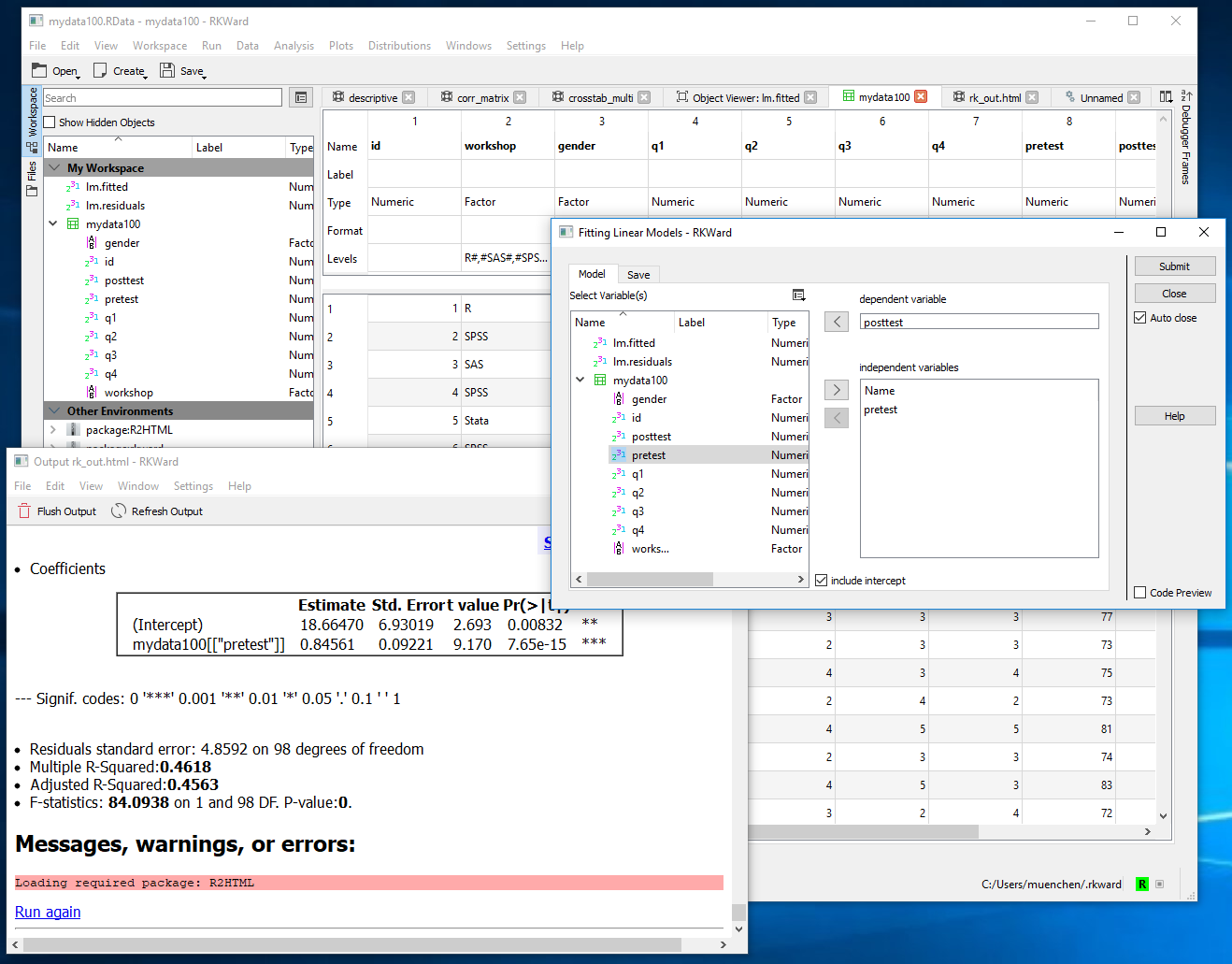
Figure 1 shows a typical RKWard session. The main control panel is the big window in the back. It has tabbed windows for each open data set and output set. RKWard makes it very easy to right-click on the tabs to detach any tabbed window. That would make it quite easy to compare two data sets side-by-side or to make full use of multiple displays.
At the top of the control panel, you’ll find the usual “File, Edit…Help” menus. Immediately below that is a toolbar containing shortcut icons. These provide a commonly used subset of the main menus, and the icons that appear there change slightly depending on your actions. The icons include: Open, Create, Save, Save Script…. The Save icon does drop down a menu, offering to save your workspace (i.e., your dataset) or your script. The “Save Script” icon is handy for saving your most recent changes to the same filename with a single click. The usual CTRL-S shortcut does the same thing.
Running plots or analyses are done as usual by making menu selections. Dialog boxes appear, and you select variables, then click an arrow icon to move them into the empty role boxes (also shown in Fig 1, right). The shortcut CTRL-click allows you to select a set of variables one at a time, as usual. Shift-click lets you select contiguous sets of variables, but a bug in the development tool RKward uses (Qt) doesn’t always show you they’re selected until you wave your mouse pointer across the selected variables. Unlike many other R GUIs, you can’t drag and drop the variables into their various roles.
When you’ve made your dialog box choices, you click “Submit” to run the step. If you want to see the R code that each dialog generates, click the “Code Preview” box in the bottom right corner of each dialog, and it will appear in the bottom of the dialog. While the code is displayed, any dialog changes you make will immediately be reflected in the code, which is very helpful when you’re learning to program. The reverse is not true since you cannot make changes to the code there. You would have to copy it and paste it into the program editor.
Most other GUIs maintain their dialog box settings within a work session, so if you wanted to do a variation of the previous step, you would simply choose it from the menus again. If you try that in RKWard, you’ll see your last round of settings have been cleared out. They are saved in the output file though. Each set of results in the output window contains a “Run again” link at the bottom of its section. Clicking that link will restore the dialog, complete with all the settings you used for that section of output.
While most dialog boxes are controlled by selecting variables from data frames, some require other types of data objects. For example, the factor analysis plug-in requires data stored in a correlation matrix. However, the correlation matrix dialog box doesn’t allow for saving the matrix, so you’d have to know how to do that using R code.
When exiting RKWard, it asks if you want to save your workspace and code (if you’ve entered any). It will automatically save your output and the dialog boxes required to make it in the file rk_out.html. This is loaded automatically in future sessions and maintains its “Run Again” capability. To save that to a different location, you can use “Workspace> Save workspace” or, on the lower set of menus, “Save> Save workspace.”
Documentation & Training
The user documentation for RKWard is located on the project’s web site. YouTube.com also offers many training videos that show how to use RKWard.
Help
R GUIs provide simple task-by-task dialog boxes, which generate much more complex code. Sometimes, that code consists of custom functions that control R’s standard ones. So, for a particular task, there is the potential for you to need help at three levels of complexity. Nearly all R GUIs provide that level of help when needed. The notable exception is the R Commander, which lacks help on the dialog boxes.
RKWard provides help files at all three levels. Each dialog box has a help button that provides a summary description, how to use the dialog box, all the GUI settings, what related functions are used, any dependencies involved, and an “About” section that provides the function’s version and its authors. Each help page also links to R’s built-in help on any functions used.
When you click on Help in a dialog, the help appears in RKWard’s main window. That comes to the front, which may cover up the dialog itself. That window contains Back, and Forward buttons, which you might think would get you back to the dialog box. So, it’s best to move the dialog to a space on your screen to allow you to read the help and see the dialog simultaneously.
The Help menu offers a search capability, but it searches only general R functions, not RKWard’s GUI-based capabilities.
Graphics
The various GUIs available for R handle graphics in several ways. Some, such as BlueSky and Deducer focus on using the popular ggplot2 package. Others, such as the R Commander, build in support for base graphics, lattice graphics, and use plug-ins for ggplot2. Still others, such as jamovi, use their own functions so they can tie them closely to the type of analysis being done.
GUIs also differ greatly in how they control the style of the graphs they generate. Ideally, you would set the style, and all graphs would follow it. That’s how jamovi works, but then jamovi is limited in the type of graphs that it does. BlueSky uses ggplot2 graphics almost exclusively, and its dialogs offer to apply “themes” from the ggthemes package.
RKWard plots are done by R’s built-in plots except for some specialty plots such as Pareto. None of them are done using lattice or ggplot2. As a result, plots of group comparisons are fairly limited.
While RKWard doesn’t let you set the style of graphics in advance, its use of R’s built-in plot functions guarantees that at least they all share one style. RKWard can save its plots to PNG, JPEG, or SVG files.
Plots in RKWard can initially be confusing, as its default highlighted variable entry box is used for pre-summarized data. For GUI users, that’s a pretty odd concept; they seldom have such data. When you enter standard un-summarized data into that field, a blank plot window results with “Error in -0.01 * height : non-numeric argument to binary operator”. Checking the “Tabulate data before plotting” box gets things working in a more standard GUI way.
RKWard’s graphics features include:
- Bar chart
- Box plot
- Cluster Analysis > Determine number of clusters
- Density plot
- Dot plot
- ECDF Plot (Empirical Cumulative Distribution Function)
- Factor Analysis > Correlation plot
- General plot
- Histogram
- Interaction plot
- Interactive BI > 1. Data Model Linker
- Interactive BI > 2. Interactive Slicer
- Interactive BI > 3. Interactive Chart
- Interactive BI > 4. Interactive Table
- Interactive BI > 5. Summary Card (KPI)
- Interactive BI > 6. Dashboard Assembler
- Interactive BI > 7. Export to HTML
- Maps > Download > Download Country Map Object
- Maps > Download > Download Global/Regional Maps
- Maps > Download > Download Municipalities
- Maps > Export Spatial Data
- Maps > Get Map Names
- Maps > Import Spatial Data
- Maps > Merge Maps
- Maps > Plot Categorical Map
- Maps > Plot Continuous Map
- Maps > Plot tidycensus map
- Maps > Recode Map Regions
- Maps > Transform Map Projection
- Network Graphs > Export Networks
- Network Graphs > Matrix to Network
- Network Graphs > Ranks to Network
- Open Street Map > Get Open Street Map Data
- Open Street Map > Plot Cartographr Map
- Pareto chart
- Pie chart
- Scatter plot
- Stem and leaf plot
- Storytelling with Data > Focus Bar Chart
- Storytelling with Data > Focus Line Chart
- Storytelling with Data > Focus Scatter Plot
- Storytelling with Data > Slopegraph
- Storytelling with Data > Dumbbell Plot
- Storytelling with Data > Big Number Summary
- Word Cloud > Create word cloud
Modeling
The way models are created and managed has a tremendous impact on both the flexibility and complexity of a user interface. The various R GUIs differ quite a lot in this regard. The simplest, and least flexible approach, is taken by jamovi which tries to do everything you might need in a single dialog box. R Commander goes the opposite direction, saving models and then offering users 25 menu selections to apply to those models. See their respective reviews on how well they succeed with each approach.
RKWard takes the simplest approach to modeling, by creating the model and offering you most of what you might want from that model in a single dialog box. The regression and ANOVA dialog boxes allow you to save models. However, there are no other menu entries devoted to model management manipulation. That struck me as a surprising choice since, in many other ways, RKWard uses the most powerful approach (e.g., code generation, programming support, object viewer, etc.).
Analysis Methods
All of the R GUIs offer a decent set of statistical analysis methods. Some also offer machine learning methods. Since this topic is so complex, I’ll simply list the methods RKWard comes with.
The first one on the Analysis menu is “Basic Statistics.” Oddly enough, by default, it doesn’t run any! I thought something had malfunctioned as I’ve never seen a stat package that didn’t offer a standard set of statistics at this stage. Just to test how it handles obvious errors, I included a factor and asked for the mean, sd, etc. This yielded the standard R messages, which beginners would find perplexing. It would have been more helpful to prevent the request by not displaying factors in that dialog box or by blocking their selection.
It turned out that the cause of my problem was that the Recode procedure had converted a numeric variable to a factor as it recoded it! The help file pointed out that there is a “Data type after recoding” setting that is set to “factor” by default. Here is a list of RKWard’s standard set of analyses, which is particularly strong in psychometrics. The Teaching menu contains duplicates of other menus, which I do not include below.
- Aiken’s Coefficients > Aiken’s H (Homogeneity)
- Aiken’s Coefficients > Aiken’s V (Content Validity)
- ANOVA for between effects
- ANOVA for mixed effects
- ANOVA within, or repeated measures, effects
- Basic Statistics
- Classical test theory > Comparing Cronbach’s alphas
- Cluster Analysis > hierarchical
- Cluster Analysis > K-means
- Cluster Analysis > model-based
- Cohen’s Kappa
- Correlation > Comparing correlations
- Correlation > Matrix Plot
- Correlation > Matrix > Kendall’s tau
- Correlation > Matrix > Pearson’s product-moment correlation
- Correlation > Matrix > Polychoric correlation
- Correlation > Matrix > Polyserial correlation
- Correlation > Matrix > Spearman’s rho
- Crosstabs N to 1
- Crosstabs N to N
- Custom Tables (expss) > Custom Table Builder
- Data Documentation Codebook > Generate Codebook
- Descriptive Statistics
- Design of Experiments (DoE) > Analyze Design
- Design of Experiments (DoE) > Fractional Factorial
- Design of Experiments (DoE) > Full Factorial Design
- Distributions: 63 dialogs cover most univariate distributions
- Factor analysis > Factor analysis
- Factor analysis > Measure of sampling adequacy (Kaiser-Meyer-Olkin)
- Factor analysis > Number of factors > Parallel analysis (Horn)
- Factor analysis > Number of factors > Scree plot
- Factor analysis > Number of factors > Very simple structure/Min ave. partial
- gt Summaries > Summary Table (gtsummary)
- gt Summaries > Survey Summary Table (gtsummary)
- Industrial Stats > Reliability > Life Data Analysis
- Industrial Stats > Reliability > Warranty Prediction
- Industrial Stats > Six Sigma > Attribute Agreement
- Industrial Stats > Six Sigma > Gage R and R
- Industrial Stats > Six Sigma > Process Capability
- Item Response Theory > Cronbach’s alpha
- Item Response Theory > Dichotomous Data > Birnbaum 3 param model
- Item Response Theory > Dichotomous Data > Linear logistic test model
- Item Response Theory > Dichotomous Data > Rasch model fit
- Item Response Theory > Dichotomous Data > Two parameter logistic model fit
- Item Response Theory > Polytomous Data > Generalized partial credit model fit
- Item Response Theory > Polytomous Data > Graded response model fit
- Item Response Theory > Polytomous Data > Linear partial credit model fit
- Item Response Theory > Polytomous Data > Linear rating scale model fit
- Item Response Theory > Polytomous Data > Partial credit model fit
- Item Response Theory > Polytomous Data > Rating scale model fit
- Item Response Theory > Tests > Andersen LR Plot (RSM, PCM)
- Item Response Theory > Tests > Goodness of Fit (Rasch)
- Item Response Theory > Tests > Item-fit statistics (Rasch, LTM, 3PM)
- Item Response Theory > Tests > Person-fit statistics (Rasch, LTM, 3PM)
- Item Response Theory > Tests > Unidimensionality check (Rasch, LTM, 3PM)
- Item Response Theory > Tests > Wald test (RSM, PCM)
- Means > t-Tests > Pairwise t-Test
- Means > t-Tests > t-Test
- Moments > Anscombe-Glynn Test of Kurtosis
- Moments > Bonett-Seier Test of Geary’s Kurtosis
- Moments > D’Agostino Test of Skewness
- Moments > Moment
- Moments > Skewness and Kurtosis
- MPT > MPTinR2
- Multidimensional scaling
- Multiple choice > Evaluate test
- Multiple Response (expss) > Define Variable Set
- Multiple Response (expss) > Multiple Response Crosstabs
- Multiple Response (expss) > Multiple Response Frequencies
- Multiple Response (expss) > Raw Counts (Pivot)
- Multivariate > Multiple CA
- Multivariate > Simple CA
- Outlier tests > Chi-squared Test for Outlier
- Outlier tests > Dixon Test
- Outlier tests > Find Outlier
- Outlier tests > Grubbs Test
- Power Analysis > ANOVA (balanced one-way)
- Power Analysis > Chi-squared test
- Power Analysis > Correlation test
- Power Analysis > General linear model
- Power Analysis > Mean of a normal distribution (known variance)
- Power Analysis > Proportion tests
- Power Analysis > t-Tests of Means
- Psychology / Social Sciences > Bayesian > Bayesian Contingency Table
- Psychology / Social Sciences > Bayesian > Bayesian Correlation
- Psychology / Social Sciences > Bayesian > Bayesian Independent T-Test
- Psychology / Social Sciences > Bayesian > Bayesian One-Way ANOVA
- Psychology / Social Sciences > Frequentist > Correlation Matrix
- Psychology / Social Sciences > Frequentist > Independent T-Test
- Psychology / Social Sciences > Frequentist > One-Way ANOVA
- Psychology / Social Sciences > Frequentist > Reliability Analysis
- Quality Control (qcc) > Process Capability
- Quality Control (qcc) > Shewhart Attributes
- Quality Control (qcc) > Shewhart Charts (Continuous)
- Regression > Linear regression
- Shiny > Exploration > Automated EDA Report
- Shiny > Exploration > Quick EDA
- Shiny > Psychometrics > Shiny Item Analysis
- Shiny > Statistics > Factoshiny (PCA/CA/MCA)
- Shiny > Statistics > Shinystan Diagnostics
- Shiny > Visualization > Esquisse
- Shiny > Visualization > Visual Explorer
- Shiny > Visualization > ggplot GUI
- Shiny > Visualization > Pivot Table
- Shiny > Visualization > Professional Dynamic
- Structural Equation Modeling (lavaan) > Fit SEM Model
- Structural Equation Modeling (lavaan) > Visualize Path Diagram
- Survey > Create survey design
- Survey > Grouped Survey Analysis (by)
- Survey > Survey GLM
- Survey > Survey Mean or Total
- Survey > Survey Quantiles
- Survey > Survey Ratio
- Survey > Survey Table
- Survey > Survey Base Plots (svyplot)
- Survey > Graphs > questionr > Bar Chart
- Survey > Graphs > questionr > Histogram
- Survey > Graphs > questionr > Boxplot
- Survey > Descriptive > Frequency Table
- Survey > Graphs > Demographic Pyramid (apyramid)
- Survey > Graphs > Animation > 1. Prepare Data
- Survey > Graphs > Animation > 2. Animated Bubble Chart
- Survey > Graphs > ggGraphs > Line Graph
- Survey > Graphs > ggGraphs > Means Graph
- Survey > Graphs > ggGraphs > Bar Diagram
- Survey > Graphs > ggGraphs > Box Plot
- Survey > Graphs > ggGraphs > Hexbin Plot
- Survey > Graphs > ggGraphs > Histogram
- Survey > Graphs > Storytelling with Data > Survey Line Graph (svyby)
- Survey > Graphs > Storytelling with Data > Survey Means Graph (Dots)
- Survey > Graphs > Storytelling with Data > Survey Bar Chart
- Survey > Graphs > Storytelling with Data > Big Number Summary
- Survival Analysis (survminer) > Cox Diagnostics
- Survival Analysis (survminer) > Cox Kaplan-Meier
- Survival Analysis (survminer) > CoxPH
- Teaching > Concordance > Cohen’s Kappa
- Teaching > Concordance > Intraclass Correlation
- Teaching > Data > Data Standardization
- Teaching > Data > Data Weighting
- Teaching > Non-parametric Tests > Chi-square goodness of fit
- Teaching > Non-parametric Tests > Friedman test for repeated measures
- Teaching > Non-parametric Tests > McNemar test of independence
- Teaching > Parametric Tests > Fisher’s F test
- Teaching > Parametric Tests > Levene’s test
- Teaching > Parametric Tests > Sample size to estimate one proportion
- Teaching > Parametric Tests > Test for comparing two proportions
- Teaching > Parametric Tests > Test for one proportion
- Teaching > Parametric Tests > Test for the variance of one population
- Teaching > Regression > Models Comparison
- Teaching > Regression > Nonlinear Regression
- Teaching > Regression > Predictions
- Text analysis > Frequency analysis
- Text analysis > Hyphenation
- Text analysis > Lexical diversity
- Text analysis > Readability
- Text analysis > Tokenizing POS tagging
- Text Mining > 1. Build and Clean Corpus
- Text Mining > 2. Inspect Corpus
- Text Mining > 3. Advanced Cleaning and Stemming
- Text Mining > 4. Frequencies and DTM Matrix
- Text Mining > 5. Word Associations
- Time Series > Box-Pierce or Ljung-Box Tests
- Time Series > Hodrick-Prescott Filter
- Time Series > KPSS Test for Stationarity
- Time Series > Phillips-Perron Test
- Variances / Scale > Nonparametric tests > Ansari-Bradley Two-Sample Exact Test
- Variances / Scale > Nonparametric tests > Ansari-Bradley Two-Sample Test
- Variances / Scale > Nonparametric tests > Flinger-Killeen Test
- Variances / Scale > Nonparametric tests > Mood Two-Sample Test
- Variances / Scale > Parametric tests > Barlett Test
- Variances / Scale > Parametric tests > F-Test
- Variances / Scale > Parametric tests > Levene’s Test
- Wilcoxon tests > Wilcoxon/Mann-Whitney
- 173 + 63 distribution dialogs = 236 analytics dialogs
Generated R Code
One of the aspects that most differentiates the various GUIs for R is the code they generate. This code can help you learn to program in R. It is also helpful for documenting the analysis steps and for reproducing and perhaps automating them. But what type of code is best for you? The base R code provided by R Commander? Tidyverse-style code provided by BlueSky Statistics? The concise functions that mimic the simplicity of one-step dialogs jamovi provides?
The RKWard developers chose to display base R code that will maximize what you will learn about R by not hiding any of the behind-the-scenes complexity involved. For example, to get the mean and standard deviation for two variables, RKWard generates this code:
local({
## Compute
vars <- rk.list (Penguins[["bill_depth_mm"]], Penguins[["bill_length_mm"]])
results <- data.frame ("Variable Name"=I(names (vars)), check.names=FALSE)
for (i in 1:length (vars)) {
	var <- vars[[i]]

	results[i, "Mean"] <- mean(var,na.rm=TRUE)
	results[i, "sd"] <- sd(var,na.rm=TRUE)

	# robust statistics
}

## Print result
rk.header ("Univariate statistics", parameters=list("Omit missing values"="yes"))

rk.results (results)
})
This might seem daunting at first, leaving a beginner to sift through it to find that mean(var, na.rm = TRUE) is the function that calculates the mean. However, someone coming from another programming language will quickly see how to code a “for” loop in R. Keep in mind that people not wanting to learn to code in R will not even see this code unless they ask to.
Support for Programmers
While I’m focusing on interfaces that include menus and dialog boxes for non-programmers, people wishing to blend that work style with programming should know that most R GUIs offer very simple R code editors. People who spend much time with R code tend to use powerful Integrated Development Environments (IDEs) like RStudio.
RKWard offers a powerful and comprehensive IDE that helps programmers write and debug code. The output from running code appears in the console window, while the output created by dialogs appears in the Output tab. The IDE features of RKWard are very similar to those of RStudio.
Its code editor, Kate, has its own open-source project, and it is jam-packed with advanced features: https://kate-editor.org/about-kate/. It supports syntax highlighting, provides hints on function arguments, offers to complete object names, and more. That’s great for people wanting to execute code, but for point-and-click users, it means that there’s a lot of added complexity.
Reproducibility & Sharing
One of the biggest challenges that GUI users face is being able to reproduce what they did. Reproducibility is useful for re-running everything on the same dataset if you find a data entry error. It’s also useful for applying your work to new datasets so long as they use the same variable names (or the software can handle changes). Some scientific journals ask researchers to submit their files (usually code and data) along with their written reports so that others can check their work.
As important a topic as it is, reproducibility is a problem for GUI users, a problem that has only recently been solved by some software developers. Most GUIs (e.g., R Commander) save only code, and it’s not code the GUI users wrote, so they also can’t read it! Others, such as jamovi and BlueSky, save the dialog box entries, providing GUI users reproducibility in their preferred form.
RKWard does save dialog box settings for you to reuse. If you execute a plot or an analysis using a dialog, then decide to do a variation on that step, choosing the dialog box again will show you one devoid of your previous choices. You might think that it has “forgotten” them. However, in the output window, each step ends with the link “Run again.” Clicking that link will make the dialog reappear, complete with your last settings filled in.
If you do “run again,” the new output will appear immediately below the existing version. That’s the most convenient approach, as you’re likely to want them close for comparison purposes, but it would be nice to have the option to have it appear at the bottom of all output.
If you wish to share your work with colleagues, you would have two choices. If they’re GUI users, you would send them your data and your RKWard output/code file. They would install RKWard, open the RKWard file, change the pointer to the new data set location, and begin work. However, output files do not contain any graphs.
If your colleagues are R programmers, you could send them your data and send them your R code. They would need to install RKWard to execute the code.
Output & Report Writing
Ideally, output should be clearly labeled, well organized, and of publication quality. It might also delve into word processing through R Markdown or LaTeX documents. Several R GUIs, such as BlueSky and jamovi, meet these requirements. See the separate reviews to see how each package works on this topic.
The labeling of RKWard’s output is done via default titles, which reflect each step well but cannot be changed in the dialog boxes. So, if you try five variations of a regression model, you’ll see five sets of output, all labeled “Linear Regression.”
The output is organized in time order only; you cannot delete any of your steps. This often results in an output file filled with unneeded results. The upper right side of the output window has a “Show TOC” link, which displays a Table of Contents. Each entry is a link that jumps you directly to that part of the output, which is very convenient. Tables of contents are commonplace for GUIs to let you re-order, rename, or delete bits of output, but none of that is possible here.
RKWard’s output quality from all GUI dialogs is very high, with nice fonts and true rich text tables. That means you can paste them into any word processor and reformat them quickly. That helps speed up your work as R output defaults to mono-spaced fonts that require additional steps to get into publication form (e.g., using functions from packages such as xtable or texreg).
RKWard now offers support for R Markdown, which allows it to save a wide variety of output file formats including Beamer, HTML, Word, Markdown, ODT, PDF, PowerPoint, RTF, DocuWiki, MediaWiki, and Vignette.
Group-By Analyses
Repeating an analysis on different groups of observations is a core task in data science. Software needs to provide an ability to select a subset one group to analyze, then another subset to compare it to. All GUIs, including RKWard, perform that task. It also needs the ability to automate such selections so that you might generate dozens of analyses, one group at a time. While this has been available in commercial GUIs for decades, only one R GUI, BlueSky, includes that feature.
Output Management
Output management deals with the software’s ability to create new data sets from the output of an analysis. That output can then be used as input for further analysis. Such data can be observation-level, such as predicted values for each observation or case. When group-by analyses are run, the output can also be model-level, such as one R-squared value for each group’s model, or parameter-level, such as the p-value for each regression parameter for each group’s model. (Saving and using models themselves is covered under “Modeling” above.)
For example, in our organization, we have 250 departments and want to see if any have a gender bias on salary. We write all 250 regression models to a data set and then search to find those whose gender parameter is significant (hoping to find none, of course).
RKWard’s modeling dialogs have the ability to save observation-level information such as predicted values and residuals. Since RKWard has such a nice spreadsheet data editor, you might expect your new variables to be saved to your original dataset, where you can view them. However, by default, they are instead saved as individual vectors.
Since RKWard lacks the ability to perform group-by processing, it has no ability to save model-level information, nor can it save parameter-level results for further analysis.
Developer Issues
The RKWard development team has created a set of tools to help R package developers to convert their work into RKWard plugins. The process consists of creating dialog boxes and determining their place on the menu structure and adding formatting to output, so that true tables appear along with quality fonts.
Conclusion
RKWard is a powerful front-end to the R language, one that provides easy point-and-click control for GUI users. People interested in learning the base R language will gain a great deal from the R code that RKWard generates. It is extremely clear R code, hiding very little within custom functions (much less than other user interfaces). Hopefully, the issue of R crashing on Macs will be remedied in the near future.
For R power users, RKWard offers a complete integrated development environment that is roughly equivalent to RStudio or Eclipse StatET.
If you want to expand your R user interface horizons, take RKWard out for a test drive and see how you like it!
For a summary of all my R GUI software reviews, see the article, R Graphical User Interface Comparison.
Acknowledgments
Thanks to Thomas Friedrichsmeier, Meik Michalke, and the RKWard team for creating RKWard and giving it away for us all to use. A special thanks to Thomas Friedrichmeier for his many suggestions that improved this article. Thanks to Alfonso Cano Robles for providing updated lists of dialogs. Also, thanks to Rachel Ladd for her editorial suggestions.