A Comparative Review of the jamovi GUI for R

by Robert A. Muenchen, updated September 2, 2024

Introduction

jamovi (spelled with a lowercase “j”) is a free and open-source graphical user interface for the R programming language. It targets beginners looking to point and click their way through analyses. It is available for Windows, Mac, Linux, and even ChromeOS. Versions are also planned for servers and tablets. This is one of a series of reviews that aim to help non-programmers choose the Graphical User Interface (GUI) for R that is best for them. Additionally, these reviews include cursory descriptions of the programming support that each GUI offers.

I have joined the BlueSky Statistics development team and written the BlueSky User Guide (online here), but you can trust this review series, as described here. All my comments below are easily verifiable. There is no perfect user interface for everyone; each GUI for R has features that appeal to different people.

Terminology

There are various definitions of user interface types, so here’s how I’ll be using the following terms. Reviewing R GUIs keeps me quite busy, so I don’t have time also to review all the IDEs, though my favorite is RStudio.

GUI = Graphical User Interface using menus and dialog boxes to avoid having to type programming code. I do not include any assistance for programming in this definition. So, GUI users are people who prefer using a GUI to perform their analyses. They don’t have the time or inclination to become good programmers.

IDE = Integrated Development Environment, which helps programmers write code. I do not include point-and-click style menus and dialog boxes when using this term. IDE users are people who prefer to write R code to perform their analyses.

Installation

The various user interfaces available for R differ quite a lot in how they’re installed. Some, such as RKWard, install in a single step. Others install in multiple steps, such as R Commander (two steps), and Deducer (up to seven steps). Advanced computer users often don’t appreciate how lost beginners can become while attempting even a simple installation. The HelpDesks at most universities are flooded with such calls at the beginning of each semester!

jamovi’s single-step installation is extremely easy and includes its own copy of R. So if you already have a copy of R installed, you’ll have two after installing jamovi. That’s a good idea, though, as it guarantees compatibility with the version of R that it uses, plus a standard R installation by itself is harder than jamovi’s. Python is also installed with jamovi, but it is used only for internal purposes. You can directly control only R through jamovi.

Plug-in Modules

When choosing a GUI, one of the most fundamental questions is: what can it do for you? What the initial software installation of each GUI gets you is covered in the Graphics, Analysis, and Modeling sections of this series of articles. Regardless of what comes built-in, it’s good to know how active the development community is. They contribute “plug-ins” that add new menus and dialog boxes to the GUI. This activity level ranges from very low (RKWard, Deducer) to very high (R Commander).

For jamovi, plug-ins are called “modules,” and they are found in the “jamovi library” rather than on the Comprehensive R Archive Network (CRAN), where R and most of its packages are found. This makes locating and installing jamovi modules especially easy.

Although jamovi is one of the most recent GUIs to appear on the R scene, it has already attracted a substantial number of developers. The list of modules at publication time is listed below. You can check the latest ones on this web page.

1. Base R – converts jamovi analyses into standard R functions
2. behaviorchange – specialized analyses and visualization tools for research and application of behavior change science
3. blandr – Bland-Altman method comparison analysis, and is also available as an R package from CRAN
4. bmtest – Better nonparametric t-test (Brunner-Munzel)
5. ClinicoPathDescriptives – descriptive functions for clinicopathological research
6. clt – Central Limit Theorem demonstrations for teaching
7. cNORMj – conventional and regression-based continuous norming methods for psychometric, biometric, and medical test construction
8. deathwatch – survival analysis
9. distrACTION – quantiles and probabilities of continuous and discrete distributions
10. endoj – instrumental variables two-stage regression
11. esci – effect sizes and confidence intervals
12. flexplot – graphically-based tools for data analysis; user supplies a formula, and the software automatically chooses the graphic
13. FoodieStats – gastronomic data analysis
14. gamlj –  general linear model, linear mixed model, generalized linear models, etc.
15. jamm – advanced mediation analysis (similar to the popular Process Macro for SAS and SPSS)
16. JAR – just-about-right data analysis
17. jeva – Evidential analyses for common statistical analyses
18. jjstatsplot – a wrapper for ggstatsplot
19. jmvbaseR – t-tests, ANOVA, correlation, and regression done using classic R functions rather than the newer ones in the jmv package
20. jmvR – makes analyses from R’s stats package usable from jamovi to help people learn basic R commands
21. jpower – power analysis for common research designs
22. jReshape – reshapes datasets long to wide or reverse
23. jsq – Bayesian methods including t-tests, ANOVAs, linear models, and contingency tables
24. jsurvival – survival module of ClinicoPath
25. jTransform – functions for common dataset transformations.
26. lsj-data – example data sets to accompany the book learning statistics with jamovi
27. MAJOR – meta-analysis based on R’s metafor package
28. MEDA – multivariate exploratory data analysis (correspondence analysis via FactoMineR)
29. meddecide – functions for inter-observer and intra-observer reliability and decision test (e.g. sensitivity, specificity, PPV, NPV)
30. medmod – basic mediation and moderation analysis
31. metaumbrella – umbrella review meta-analysis
32. moretests – adds more normality and homogeneity of variance tests
33. pathj – path analysis
34. psychoPDA – Psychometrics & post-data analysis
35. QM – analysis of data from Q-methodology
36. r-datasets – adds the standard example datasets that come with R
37. Randomizer – generate various randomized experimental designs (e.g. randomized complete block)
38. Rj – editor to run R code inside jamovi
39. rosetta – parallel use of statistical packages in teaching
40. scatr – scatter plots with marginal density, box plots, & Pareto charts
41. SEDA – Sensory Evaluation Data Analysis for perception data (via SensoMineR)
42. semlj – structural equation modeling based on lavaan
43. seolmatrix – correlations suite (e.g. tetrachoric, polychoric, intraclass, partial…)
44. SimplyAgree – flexible and robust agreement and reliability analyses
45. snowCluster – k-means, hierarchical, plus visualization
46. snowIRT – Item Response Theory
47. snowLatent – latent class analysis
48. snowRMM – Rasch Mixture Model
49. Statkat – helps you choose a statistical test
50. surveymv – survey plots
51. TOSTER – tests of equivalence for t-tests and correlation
52. ufs – tools for confidence intervals for effect sizes from R’s ufs package
53. vijMR – multiple response data analysis
54. walrus – robust descriptive stats & tests
55. ztestvis – one-sample z-test
56. jamovi Arcade – hangman & blackjack games

Some user interfaces for R, such as BlueSky and Rkward, start by double-clicking on a single icon, which is great for people who prefer not to write code. Others, such as R commander and JGR, have you start R, then load a package from your library, and then call a function to activate the GUI finally. That’s more appropriate for people looking to learn R, as those are among the first tasks they’ll have to learn anyway.

You start jamovi directly by double-clicking its icon from your desktop or choosing it from your Start Menu (i.e. not from within R itself). It interacts with R in the background; you never need to be aware that R is running.

Data Editor

A data editor is a fundamental feature in data analysis software. It puts you in touch with your data and lets you get a feel for it, if only in a rough way. A data editor is such a simple concept that you might think there would be hardly any differences in how they work in different GUIs. While there are technical differences, to a beginner, what matters the most are the differences in simplicity. Some GUIs, including BlueSky, let you create only what R calls a data frame. They use more common terminology and call it a data set: you create one, you save one, later you open one, then you use one. Others, such as RKWard, trade this simplicity for the full R language perspective: a data set is stored in a workspace. So the process goes: you create a data set, you save a workspace, you open a workspace, and choose a dataset from within it.

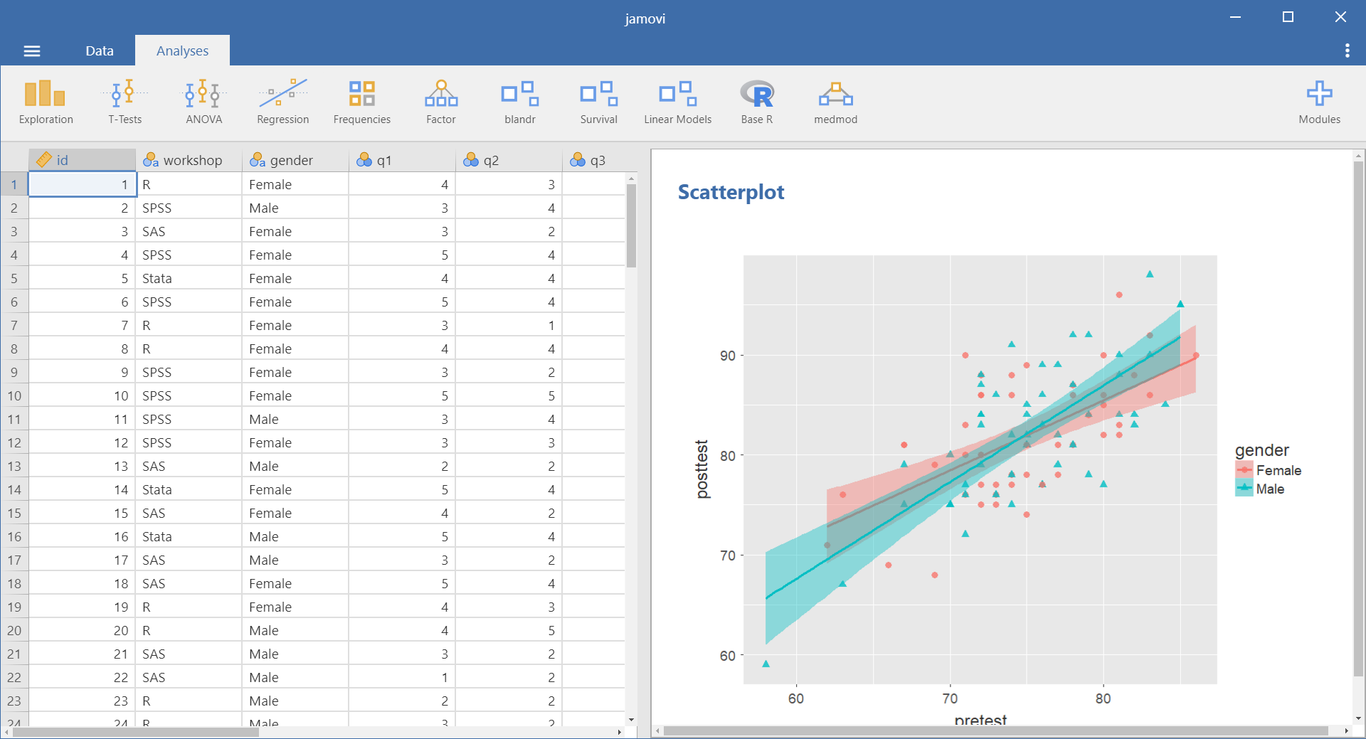
jamovi’s data editor appears at start-up (Figure 1, left) and prompts you to enter data with an empty spreadsheet-style data editor. You can start entering data immediately, though at first, the variables are simply named A, B, C….

To change metadata, such as variable names, you double-click on a name, and a window (Figure 2) will slide open from the top with settings for a variable name, description, measurement level (continuous, ordinal, nominal, or ID), data type (integer, decimal, text), variable levels (labels) and a “retain unused levels” switch. Currently, jamovi has no date format, which is a serious limitation if you deal with that popular data format.

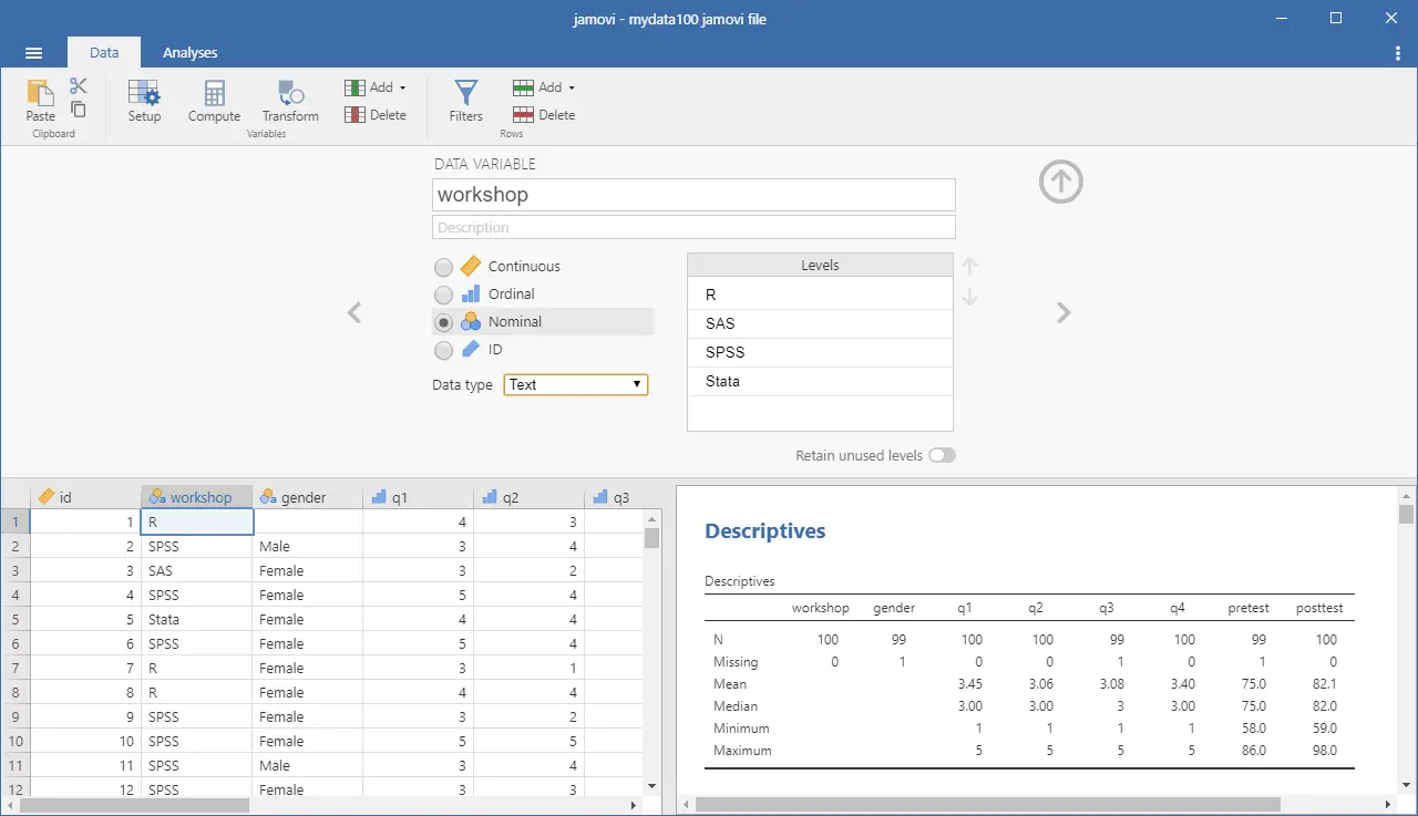
When choosing variable terminology, R GUI designers have two choices: follow what most statistics books use or instead use R jargon. The jamovi designers have opted for the statistics book terminology. For example, what jamovi calls categorical, decimal, or text are called factor, numeric, or character in R. Both sets of terms are fairly easy to learn, but given that some jamovi users may wish to learn R code, I find that choice puzzling. Changing variable settings can be done to many variables at once, which is an important time-saver.

You can enter integer, decimal, or character data in the editor right after starting jamovi. It will recognize those types and set their metadata accordingly.

To enter nominal/factor data, you are free to enter numbers, such as 1/2, and later set levels to see Male/Female appear. Or you can set it up in advance and enter the numbers, which will instantly turn into labels. That is a feature that saves time and helps assure accuracy. All data editors should offer that choice!

Adding variables or observations is as simple as scrolling beyond the set’s current limits and entering additional data. jamovi does not require “add more” buttons like some of its competitors (e.g., BlueSky) do. Adding variables or observations in between existing ones is also easy. Under the “Data” tab, there are two sets of “Add” and “Delete” buttons. The first set deals with variables, and the second with cases. You can use the first set to insert, compute, transform variables, or delete variables. The second inserts, appends, or deletes cases. These two sets of buttons are labeled “Variables” and “Rows,” but the font used is so small that I used jamovi for quite a while before noticing these labels.

Data Import

The ability to import data from a wide variety of formats is extremely important; you can’t analyze what you can’t access. Most of the GUIs evaluated in this series can open a wide range of file types and even pull data from relational databases. jamovi can’t read data from databases, but it can import the following file formats:

• Comma Separated Values (.csv)
• Open Document (.ods)
• Plain text files (.txt)
• R data files (.RData, .RDS)
• SPSS (.sav, .zsav, .por)
• SAS binary files (.sas7bdat, .xpt)
• Stata (.dta)
• JASP (.jasp)
• JSON

While jamovi doesn’t support true date/time variables, when you import a dataset that contains them, it will convert them to an integer value representing the number of days since 1970-01-01 and assign them labels in the YYYY-MM-DD format.

Data Export

The ability to export data to a wide range of file types helps when you have to use multiple tools to complete a task. Research is commonly a team effort, and in my experience, it’s rare to have all team members prefer to use the same tool. For these reasons, GUIs such as BlueSky and Deducer offer many export formats. Others, such as R Commander and RKward, can create only delimited text files.

A fairly unique feature of jamovi is that it doesn’t save just a dataset. Instead, it saves the combination of a dataset plus its associated analyses. To save just the dataset, you use the main (a.k.a. hamburger) menu to select “Export” and then “Data.”  The export formats supported are the same as those provided for import, except for JASP, JSON, and the more rarely-used ones such as SAS xpt and SPSS por and zsav:

• Comma Separated Values (.csv)
• Open Document (.ods)
• Plain text files (.txt)
• R data files (.RData, .RDS)
• SPSS (.sav)
• SAS binary files (.sas7bdat)
• Stata (.dta)

Data Management

It’s often said that 80% of data analysis time is spent preparing the data. Variables need to be transformed, recoded, or created; strings and dates need to be manipulated; missing values need to be handled; datasets need to be sorted, stacked, merged, aggregated, transposed, or reshaped (e.g. from “wide” format to “long” and back).

An essential aspect of data management is the ability to transform many variables at once. For example, social scientists need to recode many survey items, biologists need to take the logarithms of many variables. Doing these types of tasks one variable at a time is tedious. Some GUIs, such as BlueSky and R Commander, can handle nearly all of these tasks. Others, such as RKWard, handle only a few of these functions.

jamovi’s data management capabilities are a mixed bag. You can transform or recode variables, and doing so across many variables is easy. The transformations are stored in the variable itself, making it easy to see what was done by double-clicking its name. However, the R code for the transformation is not available, even with Syntax Mode turned on. In addition, all output tables are tied to the current state of the data editor. So, changing an existing variable also changes any previous output that involved that variable! Spreadsheet users will find this to be “business as usual”, but people coming from other analytic software or programming languages, may be quite surprised. Once aware of the situation, it is easy to avoid trouble by storing transformed variables under new names. That is a good policy to follow regardless.

For stacking datasets with common variables, jamovi has one of the easiest approaches I’ve ever seen. With other GUIs, you would open one data set, then the other, then conclude with the stacking operation. That leaves you wondering how to handle dozens of datasets. Importing many datasets is usually viewed as a separate problem to solve. jamovi is limited to having only one dataset open at a time, but it makes the most of it by allowing you to import many datasets at once, and it will stack them automatically!

You can also filter cases to work on a subset of your data. In previous reviews, I pointed out that, at the time, jamovi couldn’t sort, merge, aggregate, transpose, or reshape datasets. Now new add-on modules now provide those features. Only one form of a dataset can exist in a given jamovi analysis file, but major changes will pop open a new instance of jamovi complete with the new dataset form.

Menus & Dialog Boxes

The goal of pointing and clicking your way through an analysis is to save time by recognizing menu settings rather than performing the more difficult task of recalling programming commands. Some GUIs, such as BlueSky, make this easy by sticking to menu standards and using simpler dialog boxes; others, such as RKWard, use unique non-standard menus so they require more learning.

jamovi uses standard menu choices for running steps listed on the Data and Analyses tabs. Dialog boxes appear, and you select variables to place into their various roles. This is accomplished by either dragging the variable names or by selecting them and clicking an arrow located next to the particular role box. A unique feature of jamovi is that as soon as you fill in enough options to perform an analysis, its output appears instantly. There is no “OK” or “Run” button like the other GUIs reviewed here. After that, every option chosen adds to the output immediately; every option turned off is removed.

While nearly all GUIs keep your dialog box settings during your session, jamovi keeps those settings in its main “workspace” file. This allows you to return to a given analysis at a future date and try some model variations. You only need to click on the output of any analysis to have the dialog box appear to the right of it, complete with all settings intact.

Under the triple-dot menu on the upper right side of the screen, you can choose to run “Syntax Mode.” When you turn that on, the R syntax appears immediately, and when you turn it off, it vanishes just as quickly. Turning on syntax mode is the only way a jamovi user would notice that R is doing the work in the background.

Output is saved by using the standard “Menu> Save” selection.

Documentation & Training

The jamovi User Guide covers the basics of using the software. The Resources by the Community web page provides links to a helpful array of documentation and tutorials in written and video form.

Help

R GUIs provide simple task-by-task dialog boxes, which generate much more complex code. So, for a particular task, you might want to get help on 1) the dialog box’s settings, 2) the custom functions it uses (if any), and 3) the R functions that the custom functions use. Nearly all R GUIs provide all three levels of help when needed. The notable exception is the R Commander, which lacks help on the dialog boxes themselves.

jamovi doesn’t offer any integrated help files, only the documentation described in the Documentation & Training section above. The search for help can become very confusing. For example, after doing the scatterplot shown in the next section, I wondered if the scat() function offered a facet argument, normally this would be an easy question to answer. My initial attempt was to go to RStudio, load jamovi’s jmv package knowing that I routinely get help from it. However, the scat() function is not built into jamovi (or jmv); it comes in the scatr add-on module. So I had to return to jamovi and install Rj Editor module. That module lets you execute R code from within jamovi. However, running “help(scat)” yielded no result. After so much confusion, I could not find any help on that function. Hopefully, this situation will improve as jamovi matures. Of course, a non-programmer would have simply looked in the dialog box, seen the lack of a facet feature, and then assumed it did not exist.

Graphics

The various GUIs available for R handle graphics in several ways. Some, such as RKWard, focus on R’s built-in graphics. Others, such as BlueSky, focus on R’s popular ggplot graphics. GUIs also differ greatly in how they control the style of the graphs they generate. Ideally, you could set the style once, and then all graphs would follow it.

jamovi uses its own graphics functions to create plots. By default, they have the look of the popular ggplot2 package even though it uses its own functions to create them. Those functions call ggplot2 functions, so the result is the same though the code is different, should you choose to display it. jamovi is the only R GUI I have reviewed besides BlueSky that lets you set the plot style in advance, and all future plots will use that style. It does this using four popular themes. jamovi also lets you choose color palettes in advance, from a set of eight.

jamovi can save plots in PDF, PNG, SVG, and EPS formats.

Here is the selection of plots that the main installation of jamovi can create. As with all the R GUis, many of jamovi’s statistical methods also provide plots, which are not listed here.

1. Exploration> Descriptives – Bar Plot of Counts
2. Exploration> Descriptives – Bar Plot of Means
3. Exploration> Descriptives – Box Plot of Medians
4. Exploration> Descriptives – Box Plot of Means
5. Exploration> Descriptives – Density
6. Exploration> Descriptives – Histogram
7. Exploration> Descriptives – QQ Plot
8. Exploration> Descriptives – Strip Plot (called “Data”)
9. Exploration> Descriptives – Violin Plot
10. Exploration> scatr – Scatter Plot
11. Exploration> scatr – Pareto Chart
12. Exploration> scatr – Scatter with fit lines
13. Exploration> scatr – Scatter with marginal density
14. Exploration> scatr – Scatter with a marginal box plot
15. ClinicoPath> Alluvial Diagrams
16. ClinicoPath> Age Pyramid
17. ClinicoPath> Variable Tree
18. ClinicoPath> Venn Diagram
19. Flexplot> Barplot of counts
20. Flexplot> Interaction plots
21. Flexplot> Strip plot with means with confidence intervals
22. snowLatent> Profile Plot
23. snowLatent> Radar Chart
24. snowLatent> Raincloud Plot
25. snowLatent> Wordcloud
26. ufs> Diamond Plot of Means

Let’s take a look at how jamovi does scatterplots. I used the menu, “Analyses> Exploration> Scatr> Scatterplot” and filled in the variables for x- and y-axes, the group variable gender, the regression line “linear,” and then I checked the “Standard error” box. This is the plot that resulted:

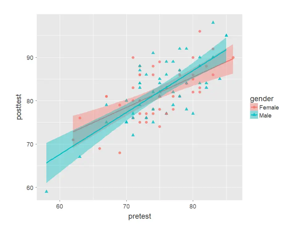
Those of you who are familiar with the ggplot2 package might already be thinking of the function call that you would use to create this common plot. However, since jamovi uses its own functions fairly exclusively, it generated the following code. Note that you will not see any code unless you activate “Syntax Mode” under the triple-dot menu.

scatr::scat(
    data = data,
    x = "pretest",
    y = "posttest",
    group = "gender",
    line = "linear",
    se = TRUE)

The flexplot plug-in adds a very useful set of plots that can be produced in small multiples, a.k.a. panel or facet plots. For example, a simple dialog box created figure 4.

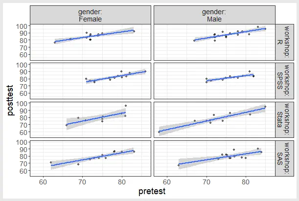
While this looks like the plot created by ggplot2 in some of the other reviews, the code used to create was this:

flexplot::flexplota(
  data = data,
  out = posttest,
  preds = pretest,
  given = vars(gender, workshop),
  line = "Regression",
  ghost = FALSE,
  JITTX = 0)

This follows the usual jamovi style of being easier to read than the usual R code used to create the plot.

However, the ability to create multiple small plots is not comprehensive. Flexplot can only create box, scatter, and bar charts (with and without confidence intervals). jamovi also lacks the ability to create large multiple plots, which reproduce the entire full-sized plot by one or more grouping factors. BlueSky Statistics and R-Instat both have that ability.

Modeling

The way statistical models (which R stores in “model objects”) are created and used is an area in which R GUIs differ the most. Some, like RKWard, use a one-step approach to modeling. That approach tries to do everything you might need in a single dialog box. This is perfect for beginners who appreciate being reminded of the various assumption tests and evaluation steps to take. But to an R programmer, that approach seems confining since R can do a lot of different tasks with model objects. However, neither SAS nor SPSS were able to save models for their first 35 years of existence, so each approach has its merits. For simple models like linear regression, standard compute statements can enter models to make predictions. Entering them manually is not much effort, and it saves you from having to learn what a model object is. However, some of the most powerful model types are essentially impossible to enter by hand, such as neural networks, random forests, and gradient-boosting machines.

Other GUIs, such as BlueSky and R Commander, do modeling using a two-step process. First, you generate and save a model, then use it for scoring new datasets, calculating model-level measures of fit or observation-level scores of influence, diagnostic plotting, testing differences between models, and so on.

jamovi follows the one-step approach. It can save predicted values, residuals, and Cook’s distance for the current dataset. However, it does not save models, so you need to use compute statements to enter a model and apply it to a new data set (or a hold-out sample) to see how effectively the model generalizes. This is great for intro statistics courses but lacks the flexibility that more advanced researchers might prefer.

Another way in which R GUIs differ is the model formula builder. Some, like JASP and RKWard, offer only the most popular model types, providing interactions and allowing you to force the y-intercept through zero. Others, such as R Commander and BlueSky, offer maximum power by including buttons to control nested factors, polynomials, splines, etc.

Jamovi keeps model formulas simple. It offers two arrows with which to add model terms. Clicking the top one adds the terms you select and all possible interactions. That can signal that you don’t have enough degrees of freedom, allowing you to remove terms. Alternatively, you can use the bottom arrow to add main effects with one click, add 2-way interactions with a second click, and so on until you have the model you need. Its model builder also includes the ability to enter predictors in blocks, obviating the need to create two models, then run a test to compare them. Since jamovi’s model builder does not offer advanced features like nested effects and splines, those models cannot be done. The model it builds is not displayed as a standard R formula, which you could modify manually.

Jamovi’s model builder also allows you to set reference levels for factors, which is typically a separate step in other R GUIs. That’s a nice touch!

If you work with datasets with a million or more cases, modeling in jamovi is quite a bit slower than the other R GUIs that pass their code directly to R. However, those other GUIs lack immediate feedback for each dialog box selection.

Analysis Methods

All of the R GUIs offer a decent set of statistical analysis methods. Some also offer machine learning methods. As you can see from the table below, jamovi offers the basics of statistical analysis. To make this list more comparable to other R GUIs, I include analyses from the Plug-in Modules for Bayesian statistics (same as those in JASP). The Plug-in Modules section above adds over 300 additional dialogs.

1. Exploration: Frequencies
2. Exploration: Descriptives
3. Independent Samples T-Test
4. Bayesian Independent Samples T-Test
5. Paired Samples T-Test
6. Bayesian Paired Samples T-Test
7. One Sample T-Test
8. Bayesian One Sample T-Test
9. ANOVA
10. Bayesian ANOVA
11. One-Way ANOVA
12. ANOVA
13. Bayesian ANOVA
14. Repeated Measures ANOVA
15. Bayesian Repeated Measures ANOVA
16. ANCOVA
17. Bayesian ANCOVA
18. MANCOVA
19. One-Way ANOVA (Non-parametric)
20. Repeated Measures ANOVA (Non-parametric)
21. Correlation Matrix
22. Partial Correlation
23. Bayesian Correlation Matrix
24. Linear Regression
25. Bayesian Linear Regression
26. Logistic Regression (2 Outcomes)
27. Logistic Regression (N Outcomes)
28. Logistic Regression (Ordinal Outcomes)
29. Proportion Test (2 Outcomes)
30. Bayesian Proportion Test (2 Outcomes)
31. Proportion Test (N Outcomes)
32. Contingency Tables, Independent
33. Contingency Tables, Paired
34. Log-Linear Regression
35. Bayesian Log-Linear Regression
36. Reliability Analysis
37. Principal Component Analysis
38. Exploratory Factor Analysis
39. Confirmatory Factor Analysis
    
    Adding the above plus 202 dialogs from add-on modules yields a total of 241 dialogs.

Generated R Code

One of the attributes that most differentiates the various GUIs for R is the code they generate. If you decide you want to save code, what type of code is best for you? The base R code as provided by the R Commander which can teach you “classic” R? The tidyverse code generated by BlueSky Statistics? The completely transparent (and complex) code provided by RKWard, which might be the best for budding R power users?

When managing data, jamovi doesn’t display any syntax. For graphics and analysis, it generates code using its own functions. So if you’re planning on learning R, you won’t be learning classic R functions, nor will you be learning the popular “tidyverse” code for R. Instead,  you’ll be learning a type of code that often looks closer to SPSS than it does to R. The advantage to this is that jamovi combines many separate R packages into one, so R programmers don’t have to find and install so many packages. The disadvantage is that you don’t learn what most people would view as R code. Of course, if you plan to only point-and-click your way through analyses, you won’t care what type of code is behind the scenes.

Is it impossible for the jamovi developers to dream of replacing common functions with their own? Not at all. The extremely popular tidyverse functions don’t do anything that classic R can’t do, they just do it in a way that its adherents view as easier. The very same thing could happen via jamovi’s jmv package of functions.

Here’s an example of code jamovi used to create a two-way ANOVA:

jmv::ANOVA(
    formula = posttest ~ gender + workshop + gender:workshop,
    data = data,
    homo = TRUE,
    postHoc = ~ workshop,
    postHocCorr = "holm",
    emMeans = ~ gender:workshop)

An R user who is familiar with analysis of variance would not recognize that code but would see that it was a single function call from one package rather than the usual half-dozen function calls from as many packages. It’s much simpler to learn, though less flexible. (Note that jmv functions do follow the tidyverse’s ability to accept piped input since the data argument is in the first position.)

Support for Programmers

Some of the GUIs reviewed in this series of articles include extensive support for programmers. For example, RKWard offers much of the power of Integrated Development Environments (IDEs) such as RStudio or Eclipse StatET. Others, such as jamovi or the R Commander, offer little more than a simple text editor.

jamovi’s main mission is to make their point-and-click GUI comprehensive. However, it does offer a plug-in module named Rj. It provides syntax highlighting (color coding), and basic code completion.

Reproducibility & Sharing

One of the biggest challenges that GUI users face is being able to reproduce their work. Reproducibility is useful for re-running everything on the same dataset if you find a data entry error. It’s also useful for applying your work to new datasets so long as they use the same variable names (or the software can handle name changes). Some scientific journals ask researchers to submit their files (usually code and data) along with their written reports so that others can check their work.

As important a topic as it is, reproducibility is a problem for GUI users, a problem that has only recently been solved by some software developers. Most GUIs (e.g. the R Commander, Rattle) save only code, but since GUI users don’t write the code, they also can’t read it or change it! Others, such as JASP, save the dialog box entries and allow GUI users reproducibility in their preferred form.

jamovi records the steps of all analyses, providing exact reproducibility. In addition, if you update a data value, all the analyses that used that variable are recalculated instantly (such manual changes are not recorded). That’s helpful, especially for people coming from Excel who expect this to happen. In addition, jamovi allows you to create a “template” that can rerun an entire set of analyses on a new dataset with the same variable names.

If you wish to share your work with colleagues who are jamovi users, you only need to give them your jamovi workspace file. It contains everything they need in a single file. This includes the dataset used (only one is possible) and any notes you have added to the output. That comprehensive package makes organization and sharing easy, but if you store multiple analyses in separate files, each will contain the dataset, which can waste space with large files.

If your colleague is an R coder, you could export your dataset to whichever file format they need and save your jamovi code. Code export is a tedious, one-analysis-at-a-time copy-paste process. While the data management code is not exportable, the dataset itself will contain the results of those transformations. Your colleague could then install the jmv package from CRAN to run your code. Note that at the moment, the Bayesian analyses cannot display their R code, but the developers are aware of the issue and plan to fix it.

Package Management

A topic related to reproducibility is package management. One of the major advantages to the R language is that it’s very easy to extend its capabilities through add-on packages. However, updates in these packages may break a previously functioning analysis. Years from now you may need to run a variation of an analysis, which would require you to find the version of R you used, plus the packages you used at the time. As a GUI user, you’d also need to find the version of the GUI that was compatible with that version of R.

Some GUIs, such as the R Commander and Deducer, depend on you to find and install R. For them, the problem is left for you to solve. Others, such as BlueSky, distribute their own version of R, all R packages, and all of its add-on modules. This requires a bigger installation file, but it makes dealing with long-term stability as simple as finding the version you used when you last performed a particular analysis. Of course, this depends on all major versions being around for long term, but for open-source software, there are usually multiple archives available to store software even if the original project is defunct.

jamovi’s approach to package management is halfway between the above two approaches. It provides nearly everything you need in a single download. This includes the jamovi interface, the jmv package, and its dependencies, R itself, and even a version of Python which is used internally. So for the base package, you’re all set. What remains to be seen is how they manage the dates for the add-on modules. While this is a current problem with long-term reproducibility, the jamovi developers are working on solving that problem.

Output & Report Writing

Ideally, output should be clearly labeled, well organized, and of publication quality. It might also delve into the realm of word processing through R Markdown, knitr, or Sweave documents. At the moment, none of the GUIs covered in this series of reviews meets all of these requirements. See the separate reviews to see how each of the other packages is doing on this topic.

The labels for each of jamovi’s analyses are provided by its menu title. The title is easy to edit, and if you do so, a text editing control bar pops up at the top, allowing you full annotation features. I assumed these were exportable into R Markdown or the newer Quarto format, but they are not. However, there is no need to learn even the simple Markdown commands since everyone knows how to use a word processing control bar.

The organization of the output is in time order only. You can delete an analysis, but you cannot move it into an order that may make more sense after you see it.

While such tables of contents are commonly used in GUIs to let you jump directly to a section, or to re-order, rename, or delete bits of output, that feature is not available in jamovi.

Those limitations aside, jamovi’s output quality is very high, with nice fonts and true rich text tables (Figure 4). Tabular output is displayed in the popular style of the American Psychological Association. That means you can right-click on any table and choose “Copy” and the formatting is retained. That really helps speed your work as R output defaults to mono-spaced fonts that require additional steps to get into publication form (e.g. using functions from packages such as xtable or texreg). You can also export an entire set of analyses to HTML, then open the nicely-formatted tables in Word.

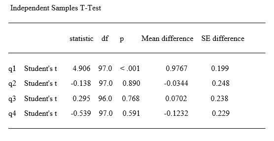
Figure 4. Output cut from jamovi & pasted into Microsoft Word. The font was changed just to show that it’s a true table.

Group-By Analyses

Repeating an analysis on different groups of observations is a core task in data science. Software needs to provide the ability to select a subset of one group to analyze, then another subset to compare it to. All the R GUIs reviewed in this series can do this task. jamovi does single-group selections using “Data> Filters”. It generates a subset that you can analyze in the same way as the entire dataset. Given jamovi’s use of immediate feedback, switching from one filter to another immediately changes the focus of every graph and analysis you’ve done. That’s rewarding, but you can’t end up with one report that contains the results for each subset. Instead, you must save each to its own file and combine the results later in a different tool (e.g., word processor, PDF merger, etc.).

Software also needs the ability to automate such selections so that you might generate dozens of analyses, one group at a time. While this has been available in commercial GUIs for decades (e.g. SPSS “split-file”, SAS “by” statement), BlueSky is the only R GUI reviewed here that includes this feature. The closest jamovi gets on this topic is to offer a “Split by” variable selection box in its Descriptives procedure.

Output Management

Early in the development of statistical software, developers tried to guess what output would be important to save to a new dataset (e.g., predicted values, factor scores), and the ability to save such output was built into the analysis procedures themselves. However, researchers were far more creative than the developers anticipated. To better meet their needs, output management systems were created and tacked on to existing tools (e.g. SAS’ Output Delivery System, SPSS’ Output Management System). One of R’s greatest strengths is that every bit of output can be readily used as input. However, with the simplification that GUIs provide, that’s a challenge.

Output data can be observation-level, such as predicted values for each observation or case.  When group-by analyses are run, the output data can also be observation-level, but now the (e.g.) predicted values would be created by individual models for each group rather than one model based on the entire original data set (perhaps with group included as a set of indicator variables).

Group-by analyses can also create model-level data sets, such as one R-squared value for each group’s model. They can also create parameter-level data sets, such as the p-value for each regression parameter for each group’s model. (Saving and using single models is covered under “Modeling” above.)

For example, in my organization, we have 250 departments and want to see if any of them have a gender bias on salary. We write all 250 regression models to a data set and then search to find those whose gender parameter is significant (hoping to find none, of course!)

While jamovi offers observation-level output, it lacks both model-level and parameter-level model summarization. BlueSky is the only R GUI reviewed here that does all three levels of output management.

Developer Issues

The jamovi development team encourages people to develop add-on modules to expand jamovi’s capabilities. It does this through a Developer’s Hub which includes a Getting Started guide. The team also offers live workshops for developers and provides the jamovi Library, which lets you publish your modules and make them easily installable by all jamovi users.

Conclusion

jamovi is a gem of a package, one that looks so good I asked the developers if they had an artist or user interface designer on the team. They don’t, but clearly, they have put a lot of thought into how to make the software beautiful and easy to use. They have also chosen their options carefully so that each analysis includes what a researcher would want to see. jamovi’s ability to save analysis templates for reuse is a feature that all GUI users will find helpful as it makes the work reusable without having to save code. Another strength to note is jamovi’s support of Bayesian analysis (borrowed from JASP).

Their creation of the jmv package is a bold move, one that promises to greatly simplify the number of separate packages a coder would need to learn. However, in so doing, they challenge the existing way of working with R. Just as the tidyverse set of commands is controversial, the jmv package is also likely to ruffle some feathers.

As nice as jamovi is, it lacks important features, including the ability to see and save data management code; the ability to handle date/time variables; the ability to perform more fundamental data management tasks; the ability to match R’s native speed when modeling with large datasets; the ability to use nested effects or splines in models; and the ability to save models so they can be tested on hold-out samples or applied to new data sets.

For a summary of all my R GUI software reviews, see the article, R Graphical User Interface Comparison.

Acknowledgments

Thanks to Jonathan Love for his suggestions that improved this review. Thanks also to Rachel Ladd, Ruben Ortiz, Christina Peterson, and Josh Price for their editorial suggestions.