by Robert A. Muenchen, updated September 4, 2024
Introduction
BlueSky Statistics’ version 10 desktop “Base” version is a free but proprietary (closed-source) graphical user interface for the R software. It focuses on beginners looking to point-and-click their way through analyses. While initially available only on Windows, the Mac version is now available. A commercial “Pro” version is also available, which includes technical support, a server version, and approximately 6% additional features (marked by a “*” below). An older version, 7.5, was open-source. That is still available for Windows only, but it lacks many features of version 10 (version 10 did immediately follow 7.5 despite the numeric gap).
This is one of a series of reviews aimed at helping non-programmers choose the best Graphic User Interface (GUI) for them. BlueSky is the only software in this series that is not open-source. While focusing on GUIs, the reviews also include a cursory description of each GUI’s programming support.
After reviewing BlueSky, I joined its development team and wrote the BlueSky User Guide (online here). However, I’m confident that you can trust this series of reviews, as I describe here. In a nutshell, the reviews describe facts that are easily verifiable. There is no perfect user interface for everyone; each GUI for R has features that appeal to different people.
Terminology
There are various definitions of user interface types, so here’s how I’ll use the following terms. Reviewing R GUIs keeps me busy, so I don’t have time to review all the IDEs, though my favorite is RStudio.
GUI = Graphical User Interface using menus and dialog boxes to avoid having to type programming code. I do not include any assistance for programming in this definition. So, GUI users prefer using a GUI to perform their analyses. They don’t have the time or inclination to become good programmers.
IDE = Integrated Development Environment, which helps programmers write code. I do not include point-and-click style menus and dialog boxes when using this term. IDE users prefer to write R code to perform their analyses.
Installation
The various user interfaces available for R differ greatly in how they’re installed. Some, such as jamovi or RKWard, install in a single step. Others, such as Deducer, install in multiple steps (up to seven, depending on your needs). Advanced computer users often don’t appreciate how lost beginners can become while attempting even a simple installation. The HelpDesks at most universities are flooded with such calls at the beginning of each semester!
The main BlueSky installation for the Apple Mac requires the installation of XQuartz. That free software allows BlueSky to display high-resolution Scalable Vector Graphics (SVG). Microsoft Windows comes with that ability so that step is not required. The BlueSky installer for Microsoft Windows and Mac provides its own embedded copy of R and 320 R packages. This simplifies the installation and ensures complete compatibility between BlueSky and its version of R. However, it also means you’ll end up with a second copy if you already have R installed. You can have BlueSky control any version of R you choose, but if the version differs too much, you may run into occasional problems. The BlueSky installation also includes a version of Python. For the moment, that is only used behind the scenes. The plan is to allow BlueSky’s GUI to control Python in the future.
Plug-in Modules
When choosing a GUI, one of the most fundamental questions is: what can it do for you? What the initial software installation of each GUI gets you is covered in this series of articles’ Graphics, Analysis, and Modeling sections. Regardless of what comes built-in, it’s good to know how active the development community is. They contribute “plug-ins” that add new menus and dialog boxes to the GUI. This level of activity ranges from very low (RKWard, Rattle, Deducer) through medium (JASP 15) to high (jamovi 43, R Commander 43).
BlueSky was a commercial package before 2018, so many of its capabilities were developed in-house. Once it became a free project, many more extensions were added, including by me. There are currently 67 extensions listed on the company website. Don’t get too carried away by the number of extensions for any R GUI since they vary significantly in capability.
There are several ways to install extensions: via file downloads, R’s main repository CRAN (Rattle, R Commander), or integrated repositories (jamovi, JASP). The integrated repository approach is by far the easiest to use. BlueSky has an integrated repository, but it comes pre-loaded with all extensions. You can then remove what you don’t need and reload them from the repository if your needs change. That approach is better for advanced users since they don’t need to add anything themselves, but it means that beginners have to see far more menus than they are likely to ever need.
Startup
Some user interfaces for R, such as jamovi or JASP, start by double-clicking on a single icon, which is great for people who prefer not to write code. Others, such as R commander or Deducer, have you start R, load a package from your library, and call a function. That’s better for people looking to learn R, as those are among the first tasks they’ll have to learn.
You start BlueSky directly by double-clicking its icon or choosing it from your Start Menu (i.e., not from within R). It interacts with R in the background; you never need to know that R is running.
Data Editor
A data editor is a fundamental feature in data analysis software. It puts you in touch with your data and lets you get a feel for it, if only in a rough way. A data editor is such a simple concept that you might think there would be hardly any differences in how they work in different GUIs. While there are technical differences, to a beginner, the differences in simplicity matter the most. Some GUIs, including jamovi, let you create only what R calls a data frame. They use more common terminology and call it a dataset: you create one, you save one, later you open one, then you use one. Others, such as RKWard, trade this simplicity for the full R language perspective: a dataset is stored in a workspace. So the process goes: you create a dataset, you save a workspace, you open a workspace, and you choose a dataset from within it.
BlueSky initially shows its screen (Figure 1) and prompts you to enter data with an empty spreadsheet-style data editor. You can start entering data immediately, though at first, the variables are named X1, X2,…. You might think you can rename them by clicking on their names, but such changes are done differently, using an approach that will be very familiar to SPSS users.
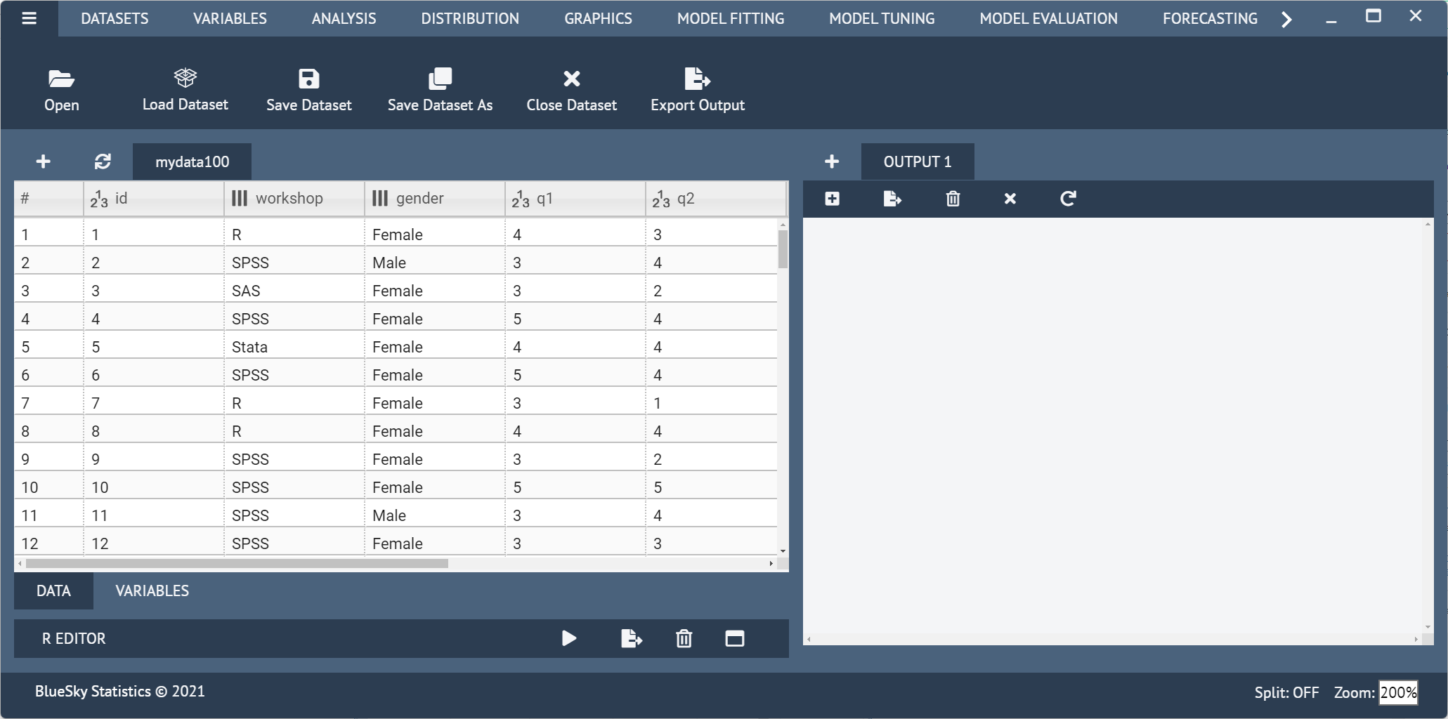
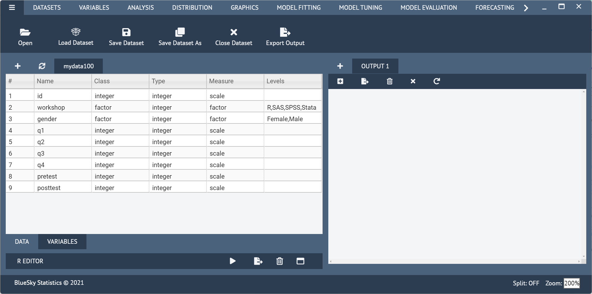
Two tabs at the bottom left of the data editor screen are labeled “Data” and “Variables.” The “Data” tab is shown by default, but clicking on the “Variables” tab takes you to a screen (Figure 2) that displays the metadata: variable names, classes, types, measurement, and for factors (categorical) the value labels.
The big advantage of SPSS is that you can simultaneously change the settings of many variables. So if you had, say, 20 variables for which you needed to set the same factor labels (e.g., 1=Strongly Disagree…5=Strongly Agree), you could do it once and then paste them into the other 19 with just a click or two. Unfortunately, that’s not implemented in BlueSky. Some of the metadata fields can be edited directly. For the rest, right-click on each variable, one at a time, to make the changes.
You can enter numeric, character, or date/time values in the editor right after starting BlueSky. They will initially all be stored as character data, displaying an “ABC” icon next to each. When you save the dataset, it looks at each variable type and converts variables that store numbers to “numeric” with a “123” icon. Date/time variables are more complex, so you must convert them using the menu item “Variables> Convert> To Date.” That uses a dialog box that allows you to choose from many different date/time formats.
Once the dataset is saved, you add rows by right-clicking any row and choosing “Insert new row above” (or below). It would be much faster if the Enter key did that automatically. Adding new variables is done using the same approach.
To enter factor data, it’s best to leave it numeric, such as 1 or 2, for male and female, then set the labels afterward. This is because once labels are set, you must enter them from drop-down menus. While that ensures no invalid values are entered, it slows down data entry.
If you instead decide to make the variable a factor before entering numeric data, it’s also best to enter the numbers as labels. It’s an oddity of R that factors are numeric inside while displaying labels that may or may not be the same as the numbers they represent.
If you have another dataset to enter, you can start the process again by clicking the “+,” and a new editor window will appear in a new tab. You can change datasets simply by clicking on its tab; its window will pop to the front for you to see. When doing analyses or saving data, the dataset that’s displayed in the editor will be used. That approach feels very natural; what you see is what you get. The ability to work with multiple datasets in a single software instance is not a feature found in all R GUIs. For example, jamovi and JASP can only work with a single dataset at a time.
The dataset is saved with the standard “File> Save Dataset As” menu. (The triple-bar menu or “hamburger” menu displayed in the current screenshots is reverting to the traditional “File” menu in the most recent version). You must save each one to its own file. While R allows multiple datasets (and other objects such as models) to be saved to a single file, BlueSky does not. Its developers chose to simplify what their users have to learn by limiting each file to a single dataset. That is a useful simplification for GUI users. If an R user sends a compound file containing many objects, BlueSky will detect it and offer to open one dataset (data frame) at a time.
on the right.
Data Import
BlueSky supports the following file formats, all automatically opened using “File> Open”:
- Comma-separated data .csv
- Pipe-separated data .psv
- Tab-separated data .tsv
- CSVY (CSV + YAML metadata header) .csvy
- SAS .sas7bdat
- SPSS .sav
- SPSS (compressed) .zsav
- Stata .dta SAS
- XPORT .xpt
- Excel .xls
- Excel .xlsx
- R syntax .R
- Saved R objects .RData, .rda
- Serialized R objects .rds
- “XBASE” database files .dbf
- Weka Attribute-Relation File Format .arff
- Fortran data no recognized extension
- Fixed-width format data .fwf
- gzip comma-separated data .csv.gz
- Apache Arrow (Parquet) .parquet
- Feather R/Python interchange format .feather
- Fast Storage .fst
- JSON .json
- Matlab .mat
- OpenDocument Spreadsheet .ods
- HTML Tables .HTML
- Shallow XML documents .XML
- YAML .yml
- Clipboard default is tsv
- Google Sheets as Comma-separated data
Additional SQL database formats are currently only available in the Windows-specific version of BlueSky and are found under the “File> Import Data” menu. These have not yet been migrated to the latest cross-platform release. The supported formats include:
- Microsoft Access
- Microsoft SQL Server
- MySQL
- Oracle
- PostgreSQL
- SQLite
Data Export
The ability to export data to a wide range of file types helps when you, or other research team members, have to use multiple tools to complete a task. Unfortunately, this is a very weak area for R GUIs. Deducer offers no data export at all, and R Commander and Rattle can export only delimited text files.
BlueSky’s comprehensive export options are the same as its import options.
Data Management
It’s often said that 80% of data analysis time is spent wrangling the data. Variables need to be transformed, recoded, or created; strings and dates need to be manipulated; missing values need to be handled; datasets need to be stacked or merged, aggregated, transposed or reshaped (e.g., from wide to long and back). A critically important aspect of data management is the ability to transform many variables simultaneously. For example, social scientists need to recode many survey items; biologists need to take the logarithms of many variables. Doing these types of tasks one variable at a time is tedious work. Some GUIs, such as jamovi and RKWard, handle only a few of these functions. Others, such as the R Commander, can handle many, but not all, of them.
BlueSky offers one of the most comprehensive sets of data management tools of any R GUI. The “Datasets” and “Variables” menus offer the following tools. Not shown is an extensive set of character and date/time functions that appear under “Compute.”
- Datasets: Aggregate
- Datasets: Compare Datasets
- Datasets: Excel Clean-up *
- Datasets: Expand
- Datasets: Find Duplicates
- Datasets: Group By: Split
- Datasets: Group By: Remove Split
- Datasets: Matching: Subject Matching *
- Datasets: Matching: Risk Set Matching *
- Datasets: Merge: Merge
- Datasets: Merge: Stack
- Datasets: Merge: Update Merge *
- Datasets: Repeating Variable Sets *
- Datasets: Reshape: Longer
- Datasets: Reshape: Wider
- Datasets: Sampling: Random Split
- Datasets: Sampling: Sample
- Datasets: Sampling: Sample, Down Sample
- Datasets: Sampling: Sample, Up Sample
- Datasets: Sampling: Stratified Sample
- Datasets: Sort: Move Variables (arbitrarily) *
- Datasets: Sort: Reorder Variables (alphabetically)
- Datasets: Sort: Sort (observations)
- Datasets: Subject Matching
- Datasets: Subset (manually enter criteria)
- Datasets: Subset: Subset by Position
- Datasets: Subset by Logic (includes logic builder) *
- Datasets: Subset: Subset by Logic
- Datasets: Transpose: Entire Dataset
- Datasets: Transpose: Selected Variables
- Variables: Bin
- Variables: Box-Cox: Add/Remove Lambda
- Variables: Box-Cox: Box-Cox Transformation
- Variables: Box-Cox: Inspect Lambda
- Variables: Box-Cox: Inverse Box-Cox
- Variables: Compute: Apply a Function to Rows
- Variables: Compute: Dummy Code
- Variables: Compute: Compute
- Variables: Compute: Conditional Compute
- Variables: Compute: Conditional Compute, Multiple
- Variables: Compute: Cumulative Statistic Variable *
- Variables: Concatenate (values)
- Variables: Convert: Date to Character
- Variables: Convert: Character to Date
- Variables: Convert: To Factor
- Variables: Convert: To Ordered Factor
- Variables: Date order check *
- Variables: Delete
- Distributions – 77 dialogs covering most distributions, plots, probabilities, etc.
- Variables: Factor Levels: Add (new levels)
- Variables: Factor Levels: Display
- Variables: Factor Levels: Drop Unused
- Variables: Factor Levels: Label NAs
- Variables: Factor Levels: Lump into Other (Automatically)
- Variables: Factor Levels: Lump into Other (Manually)
- Variables: Factor Levels: Reorder by Count
- Variables: Factor Levels: Reorder by Another Variable
- Variables: Factor Levels: Reorder by Occurance
- Variables: Factor Levels: Reorder Manually
- Variables: Fill Values Downward or Upward * (e.g. last obs value carried forward) *
- Variables: ID Variable
- Variables: Lag or Lead Variable
- Variables: Missing Values: Character / Factor
- Variables: Missing Values: Fill Values Downward or Upward *
- Variables: Missing Values: Remove NAs
- Variables: Missing Values: Numeric
- Variables: Missing Values: Use a Formula
- Variables: Missing Values, model imputation: Classification And Reg. Tree (cart)
- Variables: Missing Values, model imputation: EM Algorithm (em)
- Variables: Missing Values, model imputation: K Nearest Neighbor (knn)
- Variables: Missing Values, model imputation: Linear Model (lm)
- Variables: Missing Values, model imputation: Lasso / Ridge / Elastic-Net (en)
- Variables: Missing Values, model imputation: Multivariate Random Forest (mf)
- Variables: Missing Values, model imputation: Predictive Mean Matching (pmm)
- Variables: Missing Values, model imputation: Robust Linear Model (rlm)
- Variables: Missing Values, model imputation: Random Forest (rf)
- Variables: Missing Values, model imputation: Random Hot Deck (rhd)
- Variables: Missing Values, model imputation: Sequential Hot Deck (shd)
- Variables: Rank Variable(s)
- Variables: Recode
- Variables: Standardize
- Variables: Transform
- Refresh Data Grid
Menus & Dialog Boxes
The goal of pointing & clicking your way through analysis is to save time by recognizing menu settings rather than performing the more difficult task of recalling programming commands. Some GUIs, such as jamovi, make this easy by sticking to menu standards and using simpler dialog boxes; others, such as RKWard, use non-standard menus that are unique and require more learning.
BlueSky uses standard menu choices for running steps listed on the Graphics, Analysis, Model Fitting, or Model Tuning menus. Dialog boxes appear, and you select variables for their various roles. You drag the variable names into their roles or select them, then click an arrow next to the role box. You then can click on either a triangular Run icon to execute the step or the “</>” icon to instead write the R code to the Output window.
The output is saved not by using the standard “File > Save As” menu but instead by clicking an “Export Output” icon at the top of the Output window. From there, you can save the output in BlueSky’s native BMD “BlueSky Markdown” format, which is essentially Markdown plus dialog box settings. You can also export to R Markdown or HTML. If you exit without saving, BlueSky will prompt you to save output and syntax (if you’ve used any of the latter). If you choose, “File> Save Project” it will let you choose a folder in which to save all open datasets, outputs, and R code (if you’ve written any). Later, upon startup, all those files will open automatically.
Documentation & Training
The BlueSky User Guide, which I wrote, has over 600 pages of detailed descriptions of how to use the software. It also includes some basics on the advantages and disadvantages of various graphical and analytic methods.
The BlueSkyStatistics.com site offers training videos on how to use it. YouTube.com also offers training videos that show how to use BlueSky. I have an introductory video here.
Help
R GUIs provide simple task-by-task dialog boxes that generate much more complex code. So, for a particular task, you might want to get help on 1) the dialog box’s settings, 2) the custom functions it uses (if any), and 3) the R functions that the custom functions use. Nearly all R GUIs provide all three levels of help when needed. The notable exceptions are jamovi, which offers no help, and the R Commander, which lacks help on the dialog boxes.
BlueSky’s help level varies depending on how much help the developers think you need. Each dialog box has a help icon “?” in the upper right corner, which opens a help window. For many (not all) dialog boxes, it describes how to use the dialog box, all the GUI settings, and how the accompanying function works should you write your own code. In the top right corner of each help window is an “R” logo button that takes you to the help page for the standard R function that does the calculations (sometimes these are called directly; other times, they’re used inside BlueSky’s functions.)
I prefer a more consistent approach. There are often things in the R help files that are not implemented in BlueSky, so eliminating those situations would be less confusing. For example, in the case of a t-test, the help file describes how “formula” works, but that concept is not addressable using BlueSky’s dialog box (nor is it needed).
Graphics
The various GUIs available for R handle graphics in several ways. Some, such as RKWard, focus on R’s built-in graphics. Others, such as jamovi, use their own functions and integrate them into analysis steps. GUIs also differ greatly in how they control the style (a.k.a. theme) of the graphs they generate. Ideally, you could set the style once, and then all graphs would follow it. That’s how jamovi works, but then jamovi is limited to its custom graph functions, as nice as they may be.
Bluesky does most of its plots using the popular ggplot2 package, so that’s the code it will create if you want to learn it. BlueSky’s dialogs for creating graphs are extremely easy to use. By comparison, learning ggplot2 code can be confusing at first. Many graphical themes are included and apply to most following plots once set (some graphs are not done by ggplot2, so they ignore the theme setting). Here is the selection of plots BlueSky can create.
- Bar Chart (counts)
- Bar Chart (means, confidence intervals)
- Boxplot
- Bullseye
- Contour
- Density (counts or continuous)
- Frequency charts (factor or numeric)
- Heatmap
- Histogram
- Interaction Plot
- Line Chart
- Line Chart, stair-step plot
- Line Chart, variable order
- Maps: U.S. County Map
- Maps: U.S. State Map
- Maps: World Map
- Pie Chart
- Plot of Means
- P-P Plots
- Q-Q Plots
- ROC Curve
- Scatterplot
- Scatterplot 3D
- Scatterplot (Binned via hexagons or squares)
- Scatterplot Matrix
- Stem and Leaf Plot
- Strip Chart
- Violin Plot
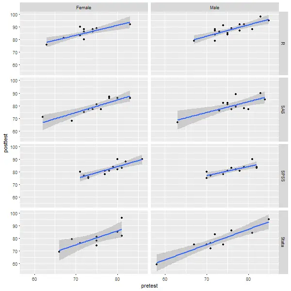
Let’s look at how BlueSky does scatterplots using R’s ggplot2 package behind the scenes. Using the dialog box, I chose only the X variable, Y variable, row facet factor, column facet factor, and the type of smoothing fit and checked a box to plot standard errors. The facets created six “small multiples” of the plot, making comparisons easy. BlueSky also includes the ability to do “large multiples” of plots by any number of other factor variables using its “Datasets> Group-by” dialog. Among R GUIs, that is currently a feature that is unique to BlueSky.
require(ggplot2);
require(ggthemes);
require(stringr);
## [Scatterplot (Points)]
ggplot(data=mydata100, aes(x=pretest,y=posttest)) +
	geom_point() +
	geom_smooth( method ="lm", alpha=1, se=TRUE,) +
	labs(x="pretest",y="posttest",
title= "Scatterplot for X axis: pretest ,Y axis: posttest ") +
	xlab("pretest") +
	ylab("posttest") +
	theme_gray() +
	theme(text=element_text(family="serif",
	face="plain",
	color="#000000",size=12,
	hjust=0.5,vjust=0.5))
Modeling
The way statistical models (which R stores in “model objects”) are created and used is an area in which R GUIs differ the most. Some, like jamovi and RKWard, use a one-step approach to modeling. That approach tries to do everything you need in a single dialog box. This is perfect for beginners who appreciate being reminded of the various assumption tests and evaluation steps. But to an R programmer, that approach seems confining since R can do many tasks with model objects. However, neither SAS nor SPSS could save models for their first 35 years of existence, so each approach has its merits. For simple models like linear regression, you can enter standard compute statements to make predictions. Entering them manually is not much effort, and it saves you from learning what a model object is. However, some of the most powerful model types, such as neural networks, random forests, and gradient-boosting machines, are essentially impossible to enter by hand.
Other GUIs, such as R Commander, do modeling using a two-step process. First, you generate and save a model. Then you use it to score new datasets, calculate model-level measures of fit or observation-level influence scores, plot diagnostics, test for differences between models, and so on.
BlueSky’s modeling approach balances flexibility and ease of use. Its “Model Fitting” dialogs save the resulting model as a model object. They contain a “Model Name” field with a helpful default name such as “LinearRegModel1”. The analyses listed under “Model Evaluation” let you use models to do things like make predictions. A complete list of the methods is shown in the next section under “Model Evaluation.”
Another way in which R GUIs differ is the model formula builder. Some, like JASP, jamovi, and RKWard, offer only the most popular model types, providing interactions and allowing you to force the y-intercept through zero. That simplicity blocks you from being able to request more advanced models. Others, such as R Commander, offer maximum power by including buttons to control nested factors, polynomials, splines, etc. Bluesky offers a combination of these approaches. Its “basic” menus offer simple dialogs for beginners, while its “advanced” dialogs include a model builder with 16 different buttons covering a wide range of model formulas. In addition, those dialogs allow you to manually type any R formula, which makes it easy for a consultant to send a model to a client via email or text.
Analysis Methods
All of the R GUIs offer a set of statistical analysis methods. Some also offer machine learning methods. As shown in the list below, BlueSky offers an extensive set of both types of models. It also offers interesting variations on machine learning. Under its “Model Fitting” dialog, it provides direct access to the most popular machine learning algorithms. If you are a beginner at machine learning, that’s where you would start. The menus call the various R functions directly, and if you display the commands, you’ll notice that each uses a slightly different syntax.
If you’re an advanced user of machine learning, you might skip directly to the “Model Tuning” menu. There you’ll find many of the same algorithms, this time controlled in a powerful and standard way using R’s caret package. You begin by choosing one of four validation methods. Within each are nine machine learning algorithms. BlueSky then passes the work to the caret package to find your optimal model.
If you do quality control or design of experiments, check out BlueSky’s Six Sigma and DOE menus, respectively. Those features make BlueSky a good alternative to Minitab and JMP.
Here is a comprehensive list of BlueSky’s methods of analysis:
- Association Rules: Generate Rules, Basket Format
- Association Rules: Item Frequency Plot, Basket Format
- Association Rules: Targeting Items, Basket Format
- Association Rules: Generate Rules, Multi-Line Format
- Association Rules: Item Frequency Plot, Multi-Line Format
- Association Rules: Targeting Items, Multi-Line Format
- Association Rules: Generate Rules, Multi-Variable Format
- Association Rules: Targeting Items, Multi-Variable Format
- Association Rules: Display Rules
- Association Rules: Plot Rules: Scatterplot
- Association Rules: Plot Rules: Two-Key Plot
- Association Rules: Plot Rules: Matrix
- Association Rules: Plot Rules: Matrix 3D
- Association Rules: Plot Rules: Graph
- Association Rules: Plot Rules: Parallel Coordinates
- Association Rules: Plot Rules: Grouped Matrix
- Association Rules: Plot Rules: Mosaic
- Association Rules: Plot Rules: Double-Decker
- Agreement: Scale: Cronbach’s Alpha
- Agreement: Scale: McDonald’s Omega
- Agreement: Method: Bland-Altman Plot
- Agreement: Method: Categorical Agreement *
- Agreement: Method: Cohen’s Kappa
- Agreement: Method: Concordance Correlation Coefficient *
- Agreement: Method: Concordance Correlation Coefficient, Multiple Raters *
- Agreement: Method: Diagnostic Testing
- Agreement: Method: Fleiss’ Kappa
- Agreement: Method: Intraclass Correlation Coefficients
- Cluster: Hierarchical
- Cluster: KMeans
- Crosstab: Crosstab
- Crosstab: Crosstab List
- Crosstab: Odds Ratios/Relative Risks, M by 2 Table *
- Correlations: Correlation Matrix
- Correlations: Pearson, Spearman
- Correlations: polychoric, polyserial
- Correlations: partial
- Correlations: semi-partial
- DOE: (Design of Experiments) DoE Overview
- DOE: Create DoE Factor Details
- DOE: Import Design Response
- DOE: Export Design
- DOE: Create Design: 2-level Screening
- DOE: Create Design: Fractional Factorial 2-level
- DOE: Create Design: Full Factorial
- DOE: Create Design: Orthogonal Array
- DOE: Create Design: D-Optimal
- DOE: Create Design: Central Composite
- DOE: Create Design: Box-Behken
- DOE: Create Design: Latin Hypercube
- DOE: Create Design: Taguchi Parameter
- DOE: Inspect Design: Inspect
- DOE: Inspect Design: Plot
- DOE: Inspect Design: Browse FrF2 Design Catalog
- DOE: Inspect Design: Browse Orthogonal Design Catalog
- DOE: Modify Design: Add/Remove Response
- DOE: Modify Design: Add Centerpoint 2-Level Design
- DOE: Analyze Design: Linear Model
- DOE: Analyze Design: Response Surface Model
- DOE: Analyze Design: Main Effects and Interaction Plots
- DOE: Analyze Design: Half Normal Plot for 2-level
- Distribution Analysis: Anderson-Darling Normality Test
- Distribution Analysis: Kolmogorov-Smirnov Normality Test
- Distribution Analysis: Shapiro-Wilk Normality Test
- Distribution Analysis: Distribution Fit P-Value *
- Distribution Analysis: Distribution Fit with GAMLSS
- Distribution Analysis: Cullen and Frey Graph
- Distributions: Continuous: Beta Probabilities
- Distributions: Continuous: Beta Quantiles
- Distributions: Continuous: Plot Beta Distribution
- Distributions: Continuous: Sample from Beta Distribution
- Distributions: Continuous: Cauchy Probabilities
- Distributions: Continuous: Plot Cauchy Distribution
- Distributions: Continuous: Cauchy Quantiles
- Distributions: Continuous: Sample from Cauchy Distribution
- Distributions: Continuous: Sample from Cauchy Distribution
- Distributions: Continuous: Chi-squared Probabilities
- Distributions: Continuous: Chi-squared Quantiles
- Distributions: Continuous: Plot Chi-squared Distribution
- Distributions: Continuous: Sample from Chi-squared Distribution
- Distributions: Continuous: Exponential Probabilities
- Distributions: Continuous: Exponential Quantiles
- Distributions: Continuous: Plot Exponential Distribution
- Distributions: Continuous: Sample from Exponential Distribution
- Distributions: Continuous: F Probabilities
- Distributions: Continuous: F Quantiles
- Distributions: Continuous: Plot F Distribution
- Distributions: Continuous: Sample from F Distribution
- Distributions: Continuous: Gamma Probabilities
- Distributions: Continuous: Gamma Quantiles
- Distributions: Continuous: Plot Gamma Distribution
- Distributions: Continuous: Sample from Gamma Distribution
- Distributions: Continuous: Gumbel Probabilities
- Distributions: Continuous: Gumbel Quantiles
- Distributions: Continuous: Plot Gumbel Distribution
- Distributions: Continuous: Sample from Gumbel Distribution
- Distributions: Continuous: Logistic Probabilities
- Distributions: Continuous: Logistic Quantiles
- Distributions: Continuous: Plot Logistic Distribution
- Distributions: Continuous: Sample from Logistic Distribution
- Distributions: Continuous: Lognormal Probabilities
- Distributions: Continuous: Lognormal Quantiles
- Distributions: Continuous: Plot Lognormal Distribution
- Distributions: Continuous: Sample from Lognormal Distribution
- Distributions: Continuous: Normal Probabilities
- Distributions: Continuous: Normal Quantiles
- Distributions: Continuous: Normal Distribution Plot with Labels *
- Distributions: Continuous: Plot Normal Distribution
- Distributions: Continuous: Sample from Normal Distribution
- Distributions: Continuous: t Probabilities
- Distributions: Continuous: t Quantiles
- Distributions: Continuous: Plot t Distribution
- Distributions: Continuous: Sample from t Distribution
- Distributions: Continuous: Uniform Probabilities
- Distributions: Continuous: Uniform Quantiles
- Distributions: Continuous: Plot Uniform Distribution
- Distributions: Continuous: Sample from Uniform Distribution
- Distributions: Continuous: Weibull Probabilities
- Distributions: Continuous: Weibull Quantiles
- Distributions: Continuous: Plot Weibull Distribution
- Distributions: Continuous: Sample from Weibull Distribution
- Distributions: Discrete: Binomial Probabilities
- Distributions: Discrete: Binomial Quantiles
- Distributions: Discrete: Binomial Tail Probabilities
- Distributions: Discrete: Plot Binomial Distribution
- Distributions: Discrete: Sample from Binomial Distribution
- Distributions: Discrete: Fit p-Value *
- Distributions: Discrete: Geometric Probabilities
- Distributions: Discrete: Geometric Quantiles
- Distributions: Discrete: Geometric Tail Probabilities
- Distributions: Discrete: Plot Geometric Distribution
- Distributions: Discrete: Sample from Geometric Distribution
- Distributions: Discrete: Hypergeometric Probabilities
- Distributions: Discrete: Hypergeometric Quantiles
- Distributions: Discrete: Hypergeometric Tail Probabilities
- Distributions: Discrete: Plot Hypergeometric Distribution
- Distributions: Discrete: Sample from Hypergeometric Distribution
- Distributions: Discrete: Negative Binomial Probabilities
- Distributions: Discrete: Negative Binomial Quantiles
- Distributions: Discrete: Negative Binomial Tail Probabilities
- Distributions: Discrete: Plot Negative Binomial Distribution
- Distributions: Discrete: Sample from Negative Binomial Distribution
- Distributions: Discrete: Poisson Probabilities
- Distributions: Discrete: Poisson Quantiles
- Distributions: Discrete: Poisson Tail Probabilities
- Distributions: Discrete: Plot Poisson Distribution
- Distributions: Discrete: Sample from Poisson Distribution
- Factor Analysis: Factor Analysis
- Factor Analysis: Principal Components
- Means: Equivalence and Minimal Effect Test
- Means: T-Test, Independent Samples
- Means: T-Test, One Sample
- Means: T-Test, Paired Samples
- Means: Legacy: Oneway ANOVA
- Means: ANCOVA
- Means: One-way ANOVA with Blocks
- Means: One-way ANOVA with Random Blocks
- Means: ANOVA, 1 and 2 Way (simplifies those models)
- Means: ANOVA, N way (includes complex model builder)
- Means: ANOVA, repeated measures, long
- Means: ANOVA, repeated measures, wide
- Means: MANOVA
- Missing Values: Output arranged in columns
- Missing Values: Output arranged in rows
- Moments: Anscombe-Glynn kurtosis test
- Moments: Bonnett-Seier kurtosis test
- Moments: D’Agostino Skewness test
- Moments: Sample moments
- Multi-dimensional scaling
- Non-parametric Tests: Chisq Test
- Non-parametric Tests: Friedman Test
- Non-parametric Tests: Kruskal-Wallis Test
- Non-parametric Tests: Wilcoxon, One Sample
- Non-parametric Tests: Wilcoxon, Independent Samples
- Non-parametric Tests: Wilcoxon, Paired Samples
- Normality test: Shapiro-Wilk
- Proportions: Binomial, Single Sample
- Proportions: Proportion Test, Independent Samples
- Proportions: Proportion Test, Single Sample
- Reliability Analysis: Cronbach’s Alpha
- Reliability Analysis: McDonald’s Omega
- Six Sigma: Six Sigma Overview
- Six Sigma: Cause and Effect
- Six Sigma: Loss Function Analysis
- Six Sigma: MSA: Gage R & R
- Six Sigma: MSA: Attribute Agreement
- Six Sigma: MSA: Gage Bias Analysis
- Six Sigma: MSA: Design MSA Study
- Six Sigma: Pareto Chart
- Six Sigma: Pareto Chart, Advanced (handles wide, long, pre-summarized)*
- Six Sigma: Process Capability: (Non-normal) *
- Six Sigma: Process Capability: QCC
- Six Sigma: Shewhart Charts: Xbar, R, S
- Six Sigma: Shewhart Charts: P, NP, C, U
- Six Sigma: Shewhart Charts: Xbar.One
- Six Sigma: Tolerance Interval *
- Six Sigma: Custom Chart
- Six Sigma: EWMA Chart
- Six Sigma: MQCC Chart
- Six Sigma: Multi-Vari Chart
- Six Sigma: Tolerance Intervals
- Summary: Descriptives
- Summary: Explore Dataset *
- Summary: Explore Variables
- Summary: Frequencies
- Summary: Frequency Plot *
- Summary: Numerical Statistical Analysis using describe
- Survival: Competing Risks, one group
- Survival: Kaplan-Meier Estimation, compare groups
- Survival: Kaplan-Meier Estimation, one group
- Time Series: Automated ARIMA
- Time Series: Exponential Smoothing
- Time Series: Holt-Winters Seasonal
- Time Series: Holt-Winters Non-seasonal
- Time Series: Plot Time Series, separate or combined
- Time Series: Plot Time Series with correlations
- Variance: Bartlett’s Test
- Variance: Levene’s Test
- Variance: Variance Test, Two Samples
- Model Builder: All N-way interactions
- Model Builder: Polynomial terms
- Model Builder: Polynomial degree
- Model Builder: df for splines
- Model Builder: B-splines
- Model Builder: Natural splines
- Model Builder: Orthogonal polynomials
- Model Builder: Raw polynomials
- Model Fitting: Contrast Display
- Model Fitting: Contrast Set
- Model Fitting: Cox, Basic
- Model Fitting: Cox, Advanced
- Model Fitting: Cox, Multiple Models *
- Model Fitting: Cox, Binary Time-Dependent Covariates *
- Model Fitting: Cox, Stratified Model *
- Model Fitting: Cox, Fine-Gray *
- Model Fitting: Decision Trees
- Model Fitting: Display Contrasts
- Model Fitting: Extreme Gradient Boosting
- Model Fitting: GLZM
- Model Fitting: IRT: Simple Rasch Model
- Model Fitting: IRT: Simple Rasch Model, multi-faceted
- Model Fitting: IRT: Partial Credit Model
- Model Fitting: IRT: Partial Credit Model, multi-faceted
- Model Fitting: IRT: Rating Scale Model
- Model Fitting: IRT: Rating Scale Model, multi-faceted
- Model Fitting: KNN
- Model Fitting: Linear Modeling
- Model Fitting: Linear Regression: Linear Regression, Basic
- Model Fitting: Linear Regression: Linear Regression, Advanced
- Model Fitting: Linear Regression: Linear Regression, Multiple Models *
- Model Fitting: Logistic Regression: Logistic Regression
- Model Fitting: Logistic Regression: Logistic Regression, Advanced
- Model Fitting: Logistic Regression: Logistic Regression, Multiple Models *
- Model Fitting: Logistic Regression: Logistic Regression, Conditional *
- Model Fitting: Mixed Models, basic
- Model Fitting: Multinomial Logit
- Model Fitting: Naive Bayes
- Model Fitting: Neural Nets: Multi-layer Perceptron
- Model Fitting: NeuralNets (i.e., the package of that name)
- Model Fitting: Nonlinear Least Squares
- Model Fitting: Ordinal Regression
- Model Fitting: Polynomial
- Model Fitting: Quantile Regression
- Model Fitting: Random Forest: Random Forest
- Model Fitting: Random Forest: Tune Random Forest
- Model Fitting: Random Forest: Random Forest: Optimal Number of Trees
- Model Fitting: Summarizing Models for Each Group
- Model Fitting: Save models
- Model Fitting: Load models
- Model Tuning: Adaboost Classification Trees
- Model Tuning: Bagged Logic Regression
- Model Tuning: Bayesian Ridge Regression
- Model Tuning: Boosted trees: gbm
- Model Tuning: Boosted trees: xgbtree
- Model Tuning: Boosted trees: C5.0
- Model Tuning: Bootstrap Resample
- Model Tuning: Decision trees: C5.0tree
- Model Tuning: Decision trees: ctree
- Model Tuning: Decision trees: rpart (CART)
- Model Tuning: K-fold Cross-Validation
- Model Tuning: K Nearest Neighbors
- Model Tuning: Leave One Out Cross-Validation
- Model Tuning: Linear Regression: lm
- Model Tuning: Linear Regression: lmStepAIC
- Model Tuning: Logistic Regression: glm
- Model Tuning: Logistic Regression: glmnet
- Model Tuning: Multi-variate Adaptive Regression Splines (MARS via earth package)
- Model Tuning: Naive Bayes
- Model Tuning: Neural Network: nnet
- Model Tuning: Neural Network: neuralnet
- Model Tuning: Neural Network: dnn (Deep Neural Net)
- Model Tuning: Neural Network: rbf
- Model Tuning: Neural Network: mlp
- Model Tuning: Random Forest: rf
- Model Tuning: Random Forest: cforest (uses ctree algorithm)
- Model Tuning: Random Forest: ranger
- Model Tuning: Repeated K-fold Cross-Validation
- Model Tuning: Robust Linear Regression: rlm
- Model Tuning: Support Vector Machines: svmLinear
- Model Tuning: Support Vector Machines: svmRadial
- Model Tuning: Support Vector Machines: svmPoly
- Model Evaluation: Add statistics to the dataset (8 measures like Cook’s D)
- Model Evaluation: ANOVA and likelihood ratio test
- Model Evaluation: Compare: Models (testing difference)
- Model Evaluation: Compare: N models (displayed in one table)
- Model Evaluation: Compare: Quantile regression models
- Model Evaluation: Compare ROC Curves
- Model Evaluation: Confidence intervals
- Model Evaluation: Fit: AIC
- Model Evaluation: Fit: BIC
- Model Evaluation: Fit: Hosmer-Lemeshow Test
- Model Evaluation: Fit: Pseudo R-squared
- Model Evaluation: Forest Plot *
- Model Evaluation: IRT: ICC Plots
- Model Evaluation: IRT: Item Fit
- Model Evaluation: IRT: Plot PI Map
- Model Evaluation: IRT: Item and Test Information
- Model Evaluation: IRT: Likelihood Ratio and Beta plots
- Model Evaluation: IRT: Personfit
- Model Evaluation: Outlier test
- Model Evaluation: Plot a Model (i.e., standard plot function applied to models)
- Model Evaluation: Predict: Model scoring
- Model Evaluation: Stepwise
- Model Evaluation: Summarize: Model statistics
- Model Evaluation: Summarize: Parameter estimates
- Model Evaluation: Summarize: Summarize a Model
- Model Evaluation: Summarize N Models
- Model Evaluation: VIF, variance inflation factor
- Sample Size: Precision: AUC
- Sample Size: Precision: Cohen’s Kappa
- Sample Size: Precision: Correlation
- Sample Size: Precision: Difference of Means
- Sample Size: Precision: ICC
- Sample Size: Precision: One Mean
- Sample Size: Precision: One Proportion
- Sample Size: Precision: Odds Ratio
- Sample Size: Precision: Risk Difference
- Sample Size: Precision: Risk Ratio
- Sample Size: Tests: ANOVA
- Sample Size: Tests: Correlation
- Sample Size: Tests: Cox Model
- Sample Size: Tests: One Mean or Paired Means
- Sample Size: Tests: One Proportion
- Sample Size: Tests: Two Group Survival
- Sample Size: Tests: Two Means
- Sample Size: Tests: Two Paired Proportions
- Sample Size: Tests: Two Proportions
Generated R Code
One of the aspects that most differentiates the various GUIs for R is the code they generate. If you decide to save code, what type of code is best for you? The base R code provided by the R Commander, which can teach you “classic” R? The concise functions that mimic the simplicity of one-step dialogs, that jamovi provides? The completely transparent (and complex) code provided by RKWard, which might be the best for budding R power users?
BlueSky writes what you might call modern R code. For data management, it uses tidyverse packages; for graphics, it uses ggplot2; and for model tuning it uses the caret package.
Here’s an example of code BlueSky wrote to do a group-by aggregation:
mySummarized <- mydata100 %>%
  dplyr::group_by(workshop,gender) %>%
  dplyr::summarize(mean_pretest = mean(pretest, na.rm = TRUE),
    mean_posttest = mean(posttest, na.rm = TRUE))
Here is an example of code BlueSky wrote to convert my repeated-measures style “long” dataset to a “wide” one. The long one had three main variables: an ID variable, a factor Time, and a measure Score. The resulting wide dataset had ID and four variables named Score_Time1, Score_Time2, Score_Time3, and Score_Time4. Here’s the code BlueSky wrote:
require (tidyr)

Bobs_wide <- mydata100 %>%
  pivot_wider(names_from = c(Time),
	      values_from = c(Score),
              names_prefix ="Score_",
              names_sort = TRUE)
Below is an example of BlueSky’s code for a simple linear regression. BlueSky even provided comments explaining each step, which is a nice touch. However, BlueSky has a set of custom functions for some statistical analyses. Those drive the actual R functions to perform calculations.
require(equatiomatic)
require(textutils)

#Creating the model
LinearRegModel1 = lm(posttest~pretest,  na.action=na.exclude, data=mydata100)

##local ({
#Display theoretical model equation and coefficients
#Display theoretical model
reg_formula = equatiomatic::extract_eq(LinearRegModel1, raw_tex = FALSE,
	 wrap = TRUE, intercept = "alpha", ital_vars = FALSE)
BSkyFormat(reg_formula)

#Display coefficients
reg_equation = equatiomatic::extract_eq(LinearRegModel1, use_coefs = TRUE,
	 wrap = TRUE,  ital_vars = FALSE, coef_digits = BSkyGetDecimalDigitSetting() )
BSkyFormat(reg_equation)

#Summarizing the model
BSky_LM_Summary_LinearRegModel1 = summary(LinearRegModel1)
BSkyFormat(BSky_LM_Summary_LinearRegModel1, singleTableOutputHeader = "Model Summary")

#Displaying the Anova table
AnovaRes = anova(LinearRegModel1 )
BSkyFormat(as.data.frame(AnovaRes), singleTableOutputHeader = "Anova table")

#Displaying sum of squares table
df = as.data.frame(AnovaRes)
totalrows = nrow(df)
regSumOfSquares = sum(df[1:totalrows - 1, 3])
residualSumOfSquares = df[totalrows, 3]
totalSumOfSquares = regSumOfSquares + residualSumOfSquares
matSumOfSquares = matrix(c(regSumOfSquares, residualSumOfSquares,
        totalSumOfSquares), nrow = 3, ncol = 1, dimnames = list(c("Sum of squares of regression",
        "Sum of squares of residuals", "Total sum of squares"),
        c("Values")))
BSkyFormat(matSumOfSquares, singleTableOutputHeader = "Sum of squares table")
Support for Programmers
Some GUIs reviewed in this series of articles include extensive support for programmers. For example, RKWard offers much of the power of Integrated Development Environments (IDEs) such as RStudio or Eclipse StatET. Others, such as jamovi or the R Commander, offer little more than a simple text editor.
While BlueSky’s main mission is to make its point-and-click GUI comprehensive, it does include a basic program editor that supports the writing and debugging of code. The code editor is hidden at the bottom left of the screen. A click on the Maximize icon will make it appear. It color-codes the commands and is smart enough to run an entire function call or pipe, even if it runs across multiple lines. It can comment and uncomment blocks of code to aid in debugging. And it has the usual find/replace and undo/redo abilities. However, that is about all it does. There is no function name completion or expanding and collapsing blocks of code (as BlueSky’s earlier Windows-only version did). RStudio and RKWard both offer much more support for coders.
However, the lack of features for coders offers a benefit to GUI users: nearly all the menus and their entries are focused on GUI use. In this regard, BlueSky is the mirror image of RKWard, which has several menus full of features that only coders use.
Reproducibility & Sharing
One of the biggest challenges that GUI users face is being able to reproduce their work. Reproducibility is useful for re-running everything on the same dataset if you find a data entry error. It’s also useful for applying your work to new datasets so long as they use the same variable names (or the software can handle name changes). Some scientific journals ask researchers to submit their files (usually code and data) along with their written reports so that others can check their work.
As important a topic as it is, reproducibility is a problem for GUI users, a problem that some software developers have only recently solved. Most GUIs (e.g., the R Commander, Rattle) save only code, but since the GUI user didn’t write the code, they also can’t read or change it! Others, such as jamovi and RKWard, save the dialog box entries and allow GUI users reproducibility in their preferred form.
BlueSky’s Output window stores the complete workflow of an analysis in both R code (hidden by default) and dialog box settings. You can also click the “+” icon in that window to add Markdown steps that allow you to provide extensive notes about what each step means. However, you have to know the Markdown commands. Those are simple, but this is an R GUI whose reason for existing is to save us from knowing code! There are plans to add a simple word-processing toolbar to let you do things like clicking a “B” icon to make something bold. Jamovi already has such a feature, though Markdown is not used to implement it.
In the free version of BlueSky, you can only reuse a workflow on a dataset with the same name used to create it. For each step you would open its dialog and rerun it. That’s a time-consuming approach which is eliminated in the commercial version. Using BlueSky Pro, you can click the ReRun icon at the top of any output window once, and it will execute all its steps. If you do not have a dataset with the same name open, it will warn you and stop. Instead, you would use “File> ReRun Output.” A dialog will open, displaying the dataset name(s) used in creating the original workflow, and the names of the dataset(s) you currently have open. You then match the previous dataset name to the new name. Repeat that process if the workflow uses multiple datasets, so BlueSky knows how to replace each one. Clicking the Run icon will apply the entire workflow to the new dataset(s). The variables do have to have the same names as those in the original workflow. The Pro version can also run reports automatically on any datasets using Windows’ Task Scheduler or Mac’s Chron command.
With GUI reproducibility, the ability to change the order of a workflow is essential. JASP has this ability, while jamovi doesn’t yet. In BlueSky, each analysis step had up/down arrows above it, allowing you to easily change the order of steps. However, as with code, changing the order can cause problems. For example, you cannot make a prediction with a model that does not yet exist!
If you wish to share your work with a colleague who also uses BlueSky, you would send them your BlueSky output file (.Bmd) and your dataset. Unlike jamovi and JASP, the dataset is not embedded in the output file. Your colleague would then install the appropriate version of BlueSky to run it. BlueSky Pro allows the storage of all related datasets, outputs, and one R program as a “project.” It then offers to export any chosen project to a zip file. Your college would then need to also have the Pro version, import the project, and then they could use it. Projects are also a way to automatically load sets of files upon startup and easily switch sets of files with a single selection.
To share your work with a colleague who uses RStudio, or a similar IDE, you would instead export your workflow to an R Markdown (.Rmd) file to send them, along with your dataset. They could install the BlueSky R package and then run all your code. The BlueSky R package is only available for download from GitHub, not on CRAN.
Package Management
A topic related to reproducibility is package management. One of the major advantages of the R language is that it’s very easy to extend its capabilities through add-on packages. However, updates in these packages may break a previously functioning analysis. Years from now, you may need to run a variation of an analysis, which would require you to find the version of R you used, plus the packages you used at the time. As a GUI user, you’d also need to find the version of the GUI that was compatible with that version of R.
Some GUIs, such as the R Commander and Deducer, depend on you to find and install R. For them, the long-term stability problem is yours to solve. Others, such as jamovi, distribute their own version of R and all R packages but not their add-on modules. This requires a bigger installation file but simplifies dealing with long-term stability. Of course, this depends on all major versions being around for the long term. Still, for open-source software (which BlueSky v10 is not), multiple archives are usually available to store software, even if the original project is defunct.
BlueSky’s approach to package management is the most comprehensive of the R GUIs reviewed here. It provides everything you need in a single download. This includes the BlueSky interface, R itself, all R packages, and all BlueSky plug-ins. If you have a problem reproducing a BlueSky analysis in the future, you only need to download the version used when you created it.
Output & Report Writing
Ideally, output should be clearly labeled, well organized, of publication quality, and include a table of contents. It might also delve into word processing using Markdown, LaTeX, or Microsoft Word. See the separate reviews to see how each package is doing on this topic.
BlueSky uses Markdown to label each output step, and you can click the “+” icon to add as much additional documentation as you like.
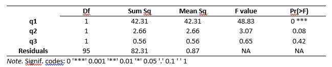
BlueSky’s output quality is very high, with nice fonts of your choosing and true rich text tables. To display them using the popular style of the American Psychological Association (see Table 1), use “Triple-dot> Settings> Output Tables” and set the output table theme to APA style, click the Save icon. That means you can copy and paste any table, and the formatting will be retained. That helps speed your work as R output defaults to mono-spaced fonts that require additional steps to get into publication form (e.g., using functions from packages such as xtable or texreg). Alternatively, you can wait until all your work is finished, export it to an HTML file, and then open it in your word processor. Unfortunately, BlueSky does not yet create Microsoft Word files directly.
The table of contents is only available in the commercial Pro version.
Group-By Analyses
Repeating an analysis on different groups of observations is a core task in data science. Software needs to provide the ability to select a subset of one group to analyze and then another subset to compare it to. All the R GUIs reviewed in this series can do this task. BlueSky does single-group selections in “Data> Subset.” It generates a subset that you can analyze in the same way as the entire dataset.
Software also needs the ability to automate such selections so that you might generate dozens of analyses or graphs, one group at a time. While this has been available in commercial GUIs for decades (e.g., SPSS split-file, SAS BY), BlueSky is the only R GUI with this feature. BlueSky automates group-by analyses under “Dataset> Group By> Split.” All the following steps will repeat for each level of the chosen factors(s). This feature is turned off via “Dataset> Group By> Remove Split.”
Output Management
Early in the development of statistical software, developers tried to guess what output would be important to save to a new dataset (e.g., predicted values, factor scores). The ability to save such output was built into the analysis procedures themselves. However, researchers were far more creative than the developers anticipated. To better meet their needs, output management systems were created and tacked on to existing tools (e.g., SAS Output Delivery System, SPSS Output Management System). One of R’s greatest strengths is that every bit of output can be readily used as input. However, with the simplification that GUIs provide, that presents a challenge.
Output data can be observation-level, such as predicted values for each observation or case. When group-by analyses are run, the output data can also be observation-level, but now the (e.g.) predicted values would be created by individual models for each group, rather than one model based on the entire original dataset (perhaps with group included as a set of indicator variables).
Group-by analyses can also create model-level datasets, such as one R-squared value for each group’s model. They can also create parameter-level datasets, such as the p-value for each regression parameter for each group’s model. (Saving and using single models is covered under “Modeling” above.)
For example, in my previous organization, we had 250 departments and wanted to see if any had a gender bias in salary. We wrote all 250 regression models to a dataset and then searched for those whose gender parameter was significant (hoping to find none, of course!).
BlueSky is the only R GUI reviewed here that does all three levels of output management. To use this function, choose “Model Fitting> Summarizing models for each group,” then specify the model and the grouping factor. It automatically creates three datasets, one at each level of analysis. This ability works only with regression, ANOVA, and multinomial logistic models. More are planned for future versions. This feature is in the older Windows-only version but has not yet been migrated to the new cross-platform version.
Developer Issues
Anyone is welcome to add new features to BlueSky. The steps are covered on the website: https://www.blueskystat.net/Development/Extending-BlueSky-Statistics.html.
Conclusion
BlueSky Statistics offers an extensive set of easy tools for a point-and-click user. It should be on your list of data science software to try, especially if you’re interested in the R language that drives its analyses. For a summary of all my R GUI software reviews, see R Graphical User Interface Comparison. The Mayo Clinic’s evaluation of many data science software packages, including BlueSky, is available here.
Acknowledgments
Thanks to the BlueSky team, who have done much hard work and made nearly all of their work free (though not open source in the latest release). Thanks to Rachel Ladd, Ruben Ortiz, Christina Peterson, and Josh Price for their editorial suggestions.